Jacobian Conjecture for Baby
An illustrated guide to a famous problem in mathematics, beginning with the basic ideas and following the story through July 2026. The original question lasted 87 years; one important part of it remains open.
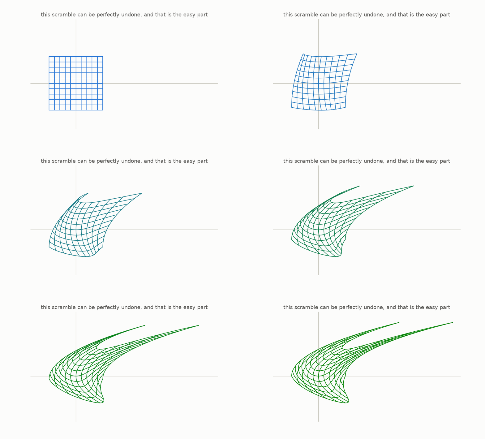
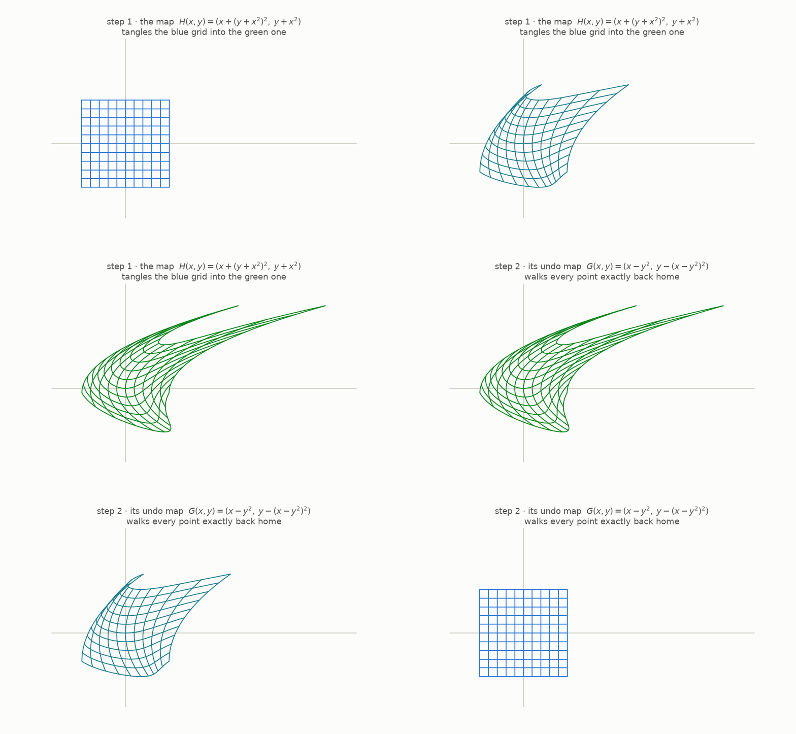
The animation shows a flat grid bending into a curved shape. At first glance, the original grid seems to have been scrambled beyond repair.
It has not. This particular bending can be undone exactly. Another simple rule sends every point back to its starting place, so no information disappears.
In 1939, the mathematician Ott-Heinrich Keller asked whether a broad class of maps behaved this way. The question became a well-known unsolved problem. Over the years, several proposed proofs were published, but each one was later found to contain a mistake.
The problem remained open for 87 years. A result announced in July 2026 settled it in dimensions three and higher, although not in the way people had expected. The original two-dimensional case is still open.
This article develops the story from the beginning, with no mathematical background assumed. Each chapter adds one idea and ties it to a picture. The last chapter gives simple arithmetic and exact computer checks for the 2026 counterexample.
(The supporting material is available in an open repository: github.com/muchmirul/conjectures. It includes the figure code and tests for the mathematical claims used here.)
Chapters 1 through 8 introduce the necessary ideas. Chapter 9 puts them together as Keller’s question, and chapters 10 through 12 explain the evidence, the obstacles, and the eventual counterexample.
1 · Functions are machines
We begin with the meaning of the word “function.”
A function can be pictured as a machine: put in a number, follow its rule, and receive another number.
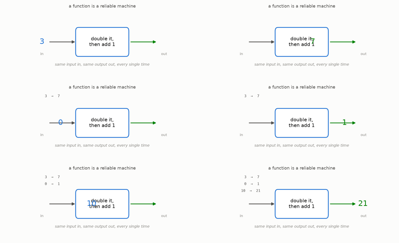
The machine in the picture doubles its input and then adds 1. An input of 3 becomes 7, an input of 0 becomes 1, and an input of 10 becomes 21.
For a rule to be a function, every allowed input must have an output, and a given input must always lead to the same output. There is no random choice between different answers.
There is another way to picture the same rule. Rather than sending numbers through one at a time, imagine that the function moves all the numbers on the number line together.
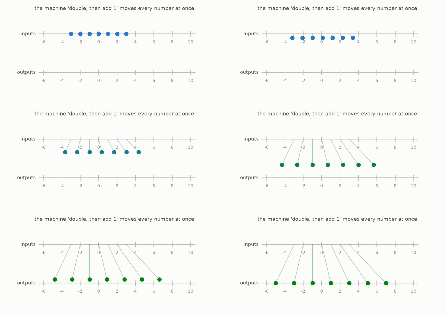
The machine has not changed; only the viewpoint has. A function can be seen as a rule that moves the whole line. Later, the same picture will be used for larger spaces.
We need one small piece of notation. Mathematicians often name a function with a letter such as $f$ and write the rule like this:
$$ f(x) = 2x + 1. $$This says that the function named $f$ takes an input, temporarily called $x$, doubles it, and adds 1. The letter $x$ simply stands for whichever input is being used.
Keep in mind: a function assigns one definite output to each input. It can also be pictured as moving all of its inputs at the same time.
2 · The undo machine
Once a machine has moved the numbers, we can ask whether another machine can move them back. This question about reversing a rule will run through the rest of the article.
For example, doubling sends 3 to 6, while halving sends 6 back to 3. If doubling is followed by halving, every number returns to where it began.
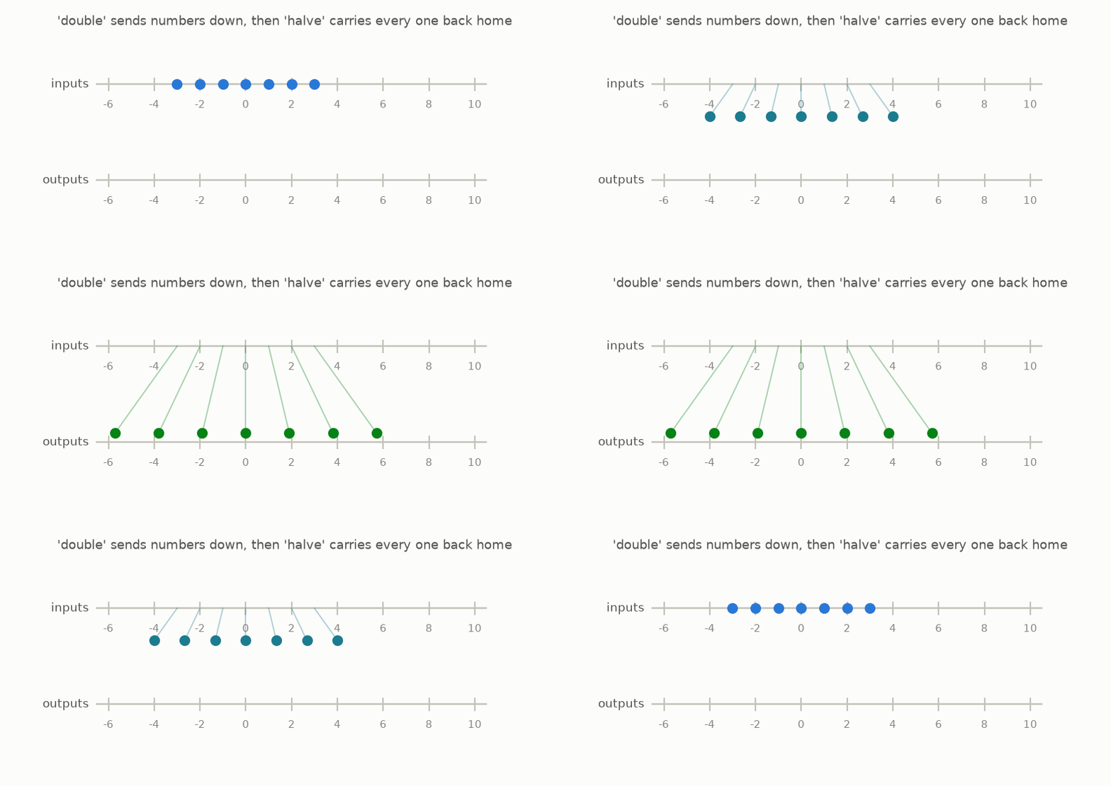
A second function that restores every original input is called an inverse. In the machine picture, it is the undo machine. Doubling and halving form one pair; adding 5 and subtracting 5 form another.
Now compare that with the rule “square the input,” meaning multiply the number by itself.
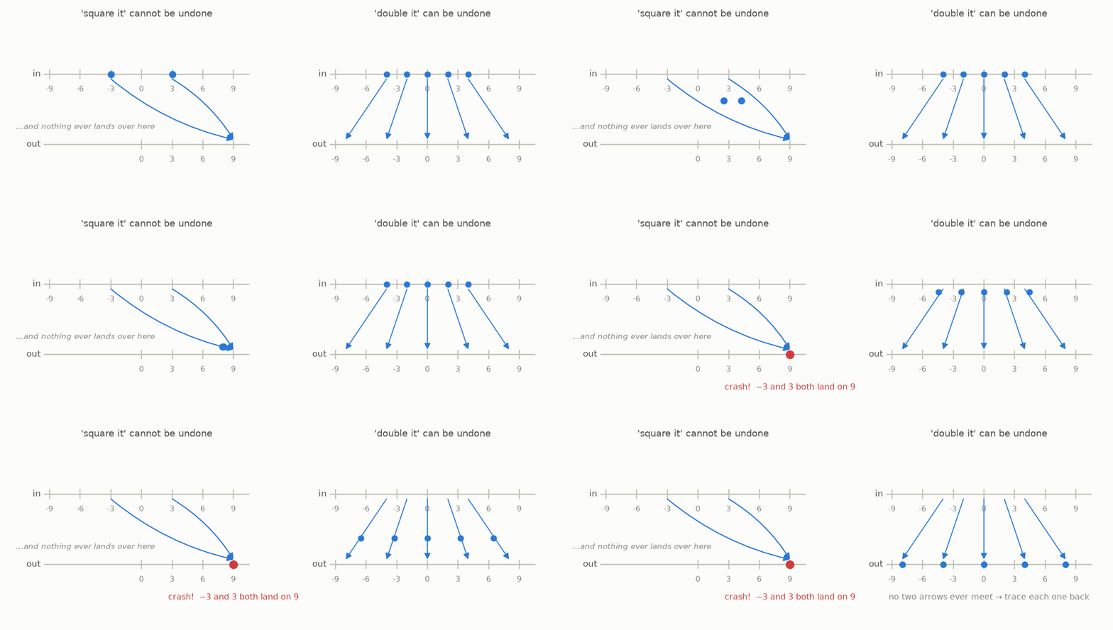
Both −3 and 3 are sent to 9. If we begin at 9 and try to reverse the rule, there is no way to tell which input was used. The sign of the original number has been lost.
Two kinds of failure prevent an undo machine from existing:
- Collisions: different inputs arrive at the same output. Squaring, for example, sends both −3 and 3 to 9.
- Gaps: some possible outputs are never reached. Squaring real numbers never produces −4.
When there are no collisions and no gaps, each output has one and only one starting point. Following that unique path backward defines the inverse.
(The standard terms are injective for “no collisions,” surjective for “no gaps,” and invertible when both conditions hold. The informal phrases will be enough for the pictures, but these are the names used in mathematics.)
Keep in mind: a function can be reversed when every output comes from exactly one input. A collision loses information, while a gap leaves the inverse with no answer.
3 · Polynomials
Functions may follow many kinds of rules. Keller’s question concerns one particular family: rules assembled from addition and multiplication.
Start with an input $x$, along with ordinary fixed numbers. Build new pieces by adding or multiplying pieces already available. A rule made by finitely many such steps is called a polynomial.
- $2x + 1$ first doubles the input and then adds one, so it is a polynomial.
- $x^2$ means $x$ multiplied by $x$, so it is also a polynomial.
- $x^3 - 2x$ combines repeated multiplication with addition of a negative number, and is another polynomial.
Their graphs appear below. The horizontal position gives the input $x$, and the height of each curve gives the corresponding output.
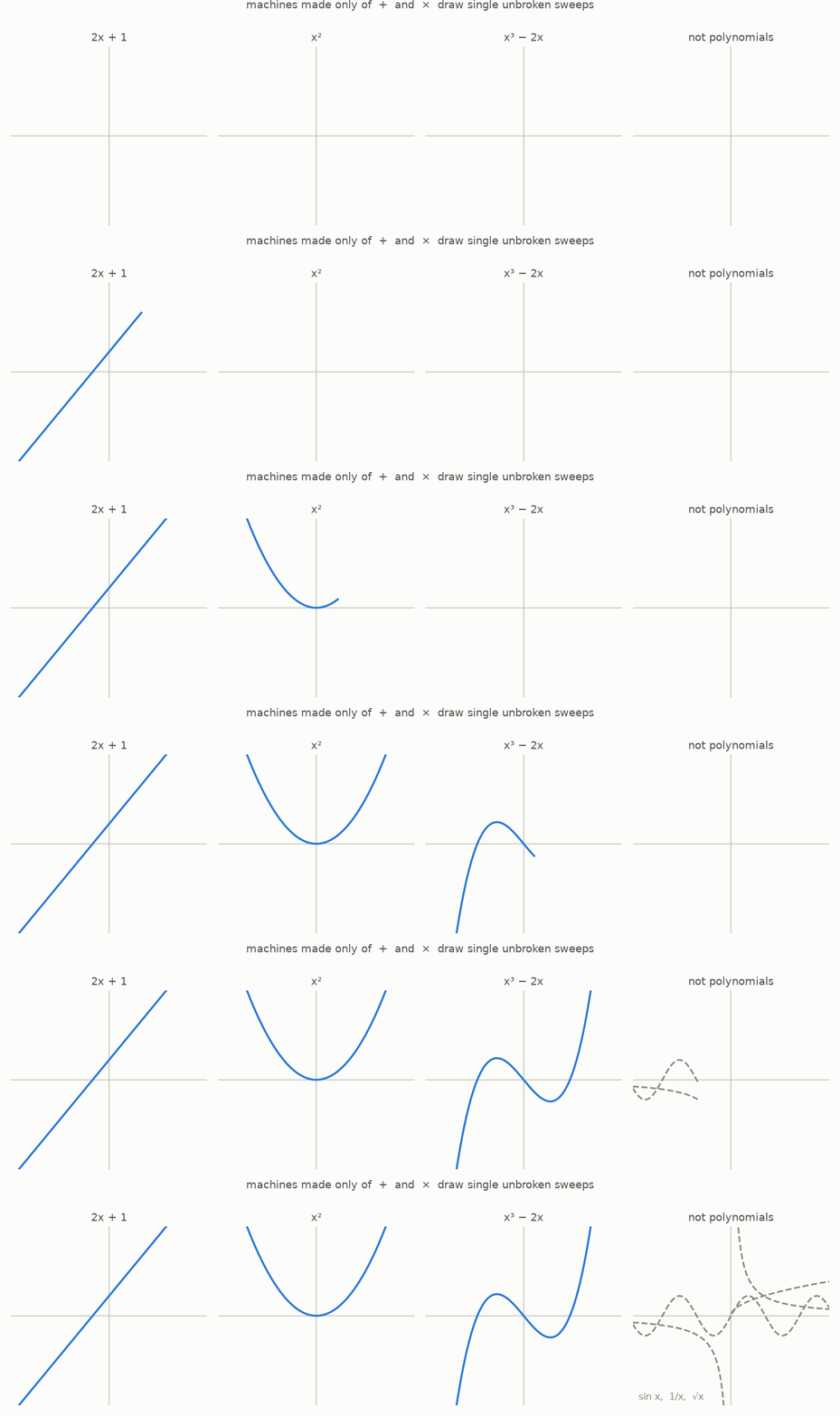
The dashed gray curves, $\sin x$, $1/x$, and $\sqrt{x}$, are not polynomials. They require operations beyond a finite list of additions and multiplications, such as division by the input, taking a root, or an infinite construction.
Polynomials are useful here because their values and their algebra can be worked out exactly in finitely many steps. They do not depend on numerical approximation or an infinite series. That makes individual examples especially easy to check.
Keller’s problem is striking partly because it asks about these concrete, finite rules, yet resisted proof for decades.
We will also use the word degree. It means the largest power that appears in a polynomial. For instance, $x^3 - 2x$ has degree 3. Degree returns in chapter 10.
Keep in mind: a polynomial is a finite rule built from numbers and inputs using addition and multiplication. Its degree is the largest power appearing in it.
4 · Maps of the plane
Functions of one number were the starting point. We now let a machine take a point as its input.
A point in the plane is described by a pair $(x, y)$: one number tells how far to move sideways and the other how far to move vertically. A plane map takes such a pair and returns another pair. It therefore has two output slots, and either slot may use both input numbers:
$$ F(x, y) = (\;\underbrace{\text{rule using } x, y}_{\text{first slot}}\;,\;\; \underbrace{\text{rule using } x, y}_{\text{second slot}}\;) $$Chapter 1 pictured a function moving a whole number line. In the same way, a plane map moves the whole plane. Drawing a grid makes that movement visible.
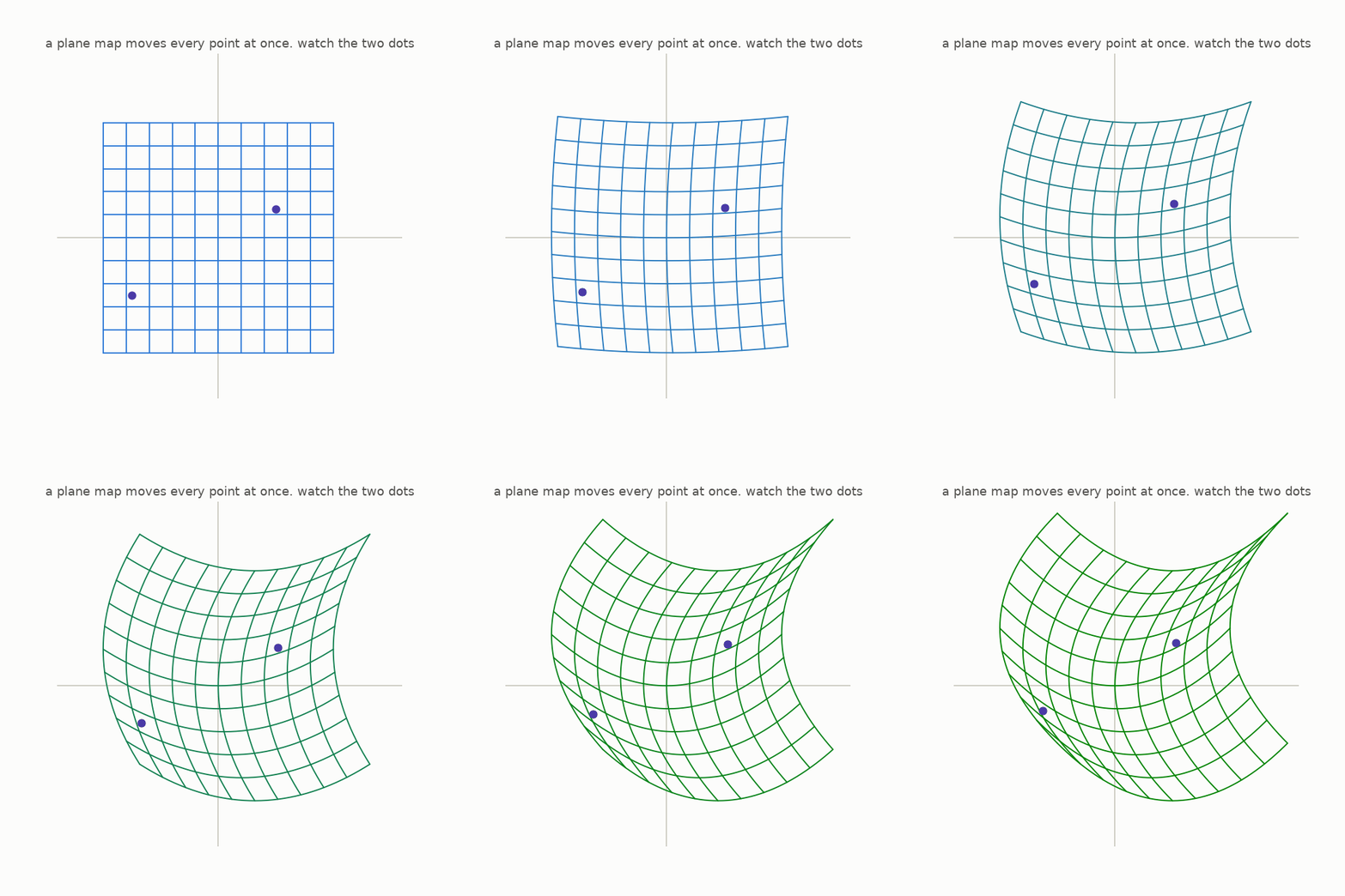
The grid behaves like marks drawn on a flexible sheet. The two highlighted dots are sample points: the map picks each one up at $(x, y)$ and places it at $F(x, y)$.
The next figure compares six basic maps of the plane.
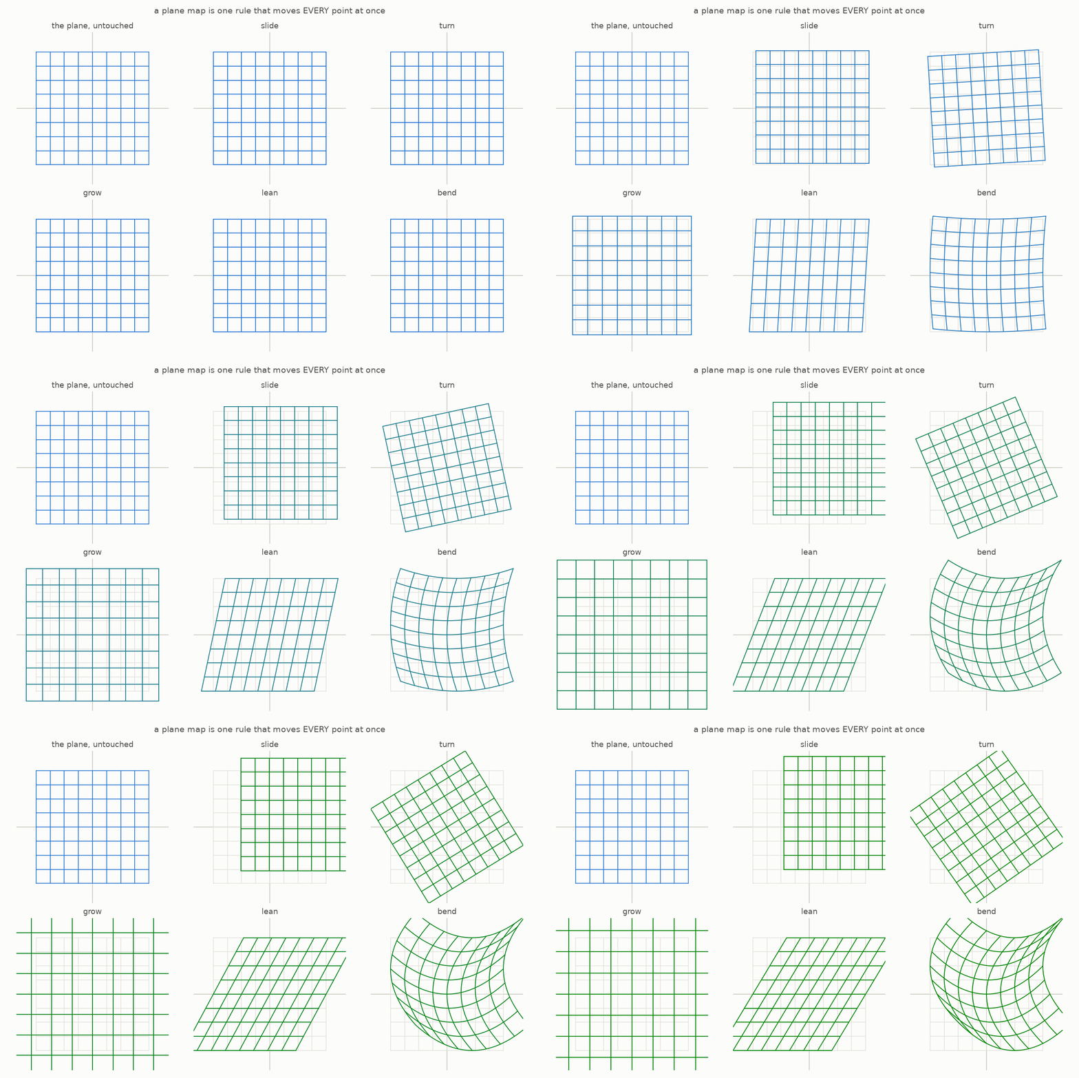
Sliding, turning, growing, and leaning leave every grid line straight. The last panel bends the lines because its rule contains $x^2$ and $y^2$. Squaring, introduced in chapter 3, is what produces the curvature.
A polynomial map of the plane has two output rules, both of them polynomials in $x$ and $y$. They use only addition and multiplication. The bend above, $F(x, y) = \left(x + \tfrac{1}{4}y^2,\; y + \tfrac{1}{4}x^2\right)$, is one example.
From this point on, the article focuses on polynomial maps of flat spaces.
Keep in mind: a plane map moves every point in the plane. It is a polynomial map when each output coordinate is built from the input coordinates using only addition and multiplication.
5 · Straight maps and the area factor
Before studying maps that bend the grid, we need one measurement from maps that keep it straight. This measurement will later be applied under the microscope.
Some plane maps keep grid lines straight, parallel, and evenly spaced, while leaving the center fixed. Mathematicians call these linear maps; here we will also call them straight maps. The turns, grows, squeezes, and leans from the previous chapter are examples.
In each panel, watch the yellow square. It begins with area 1.
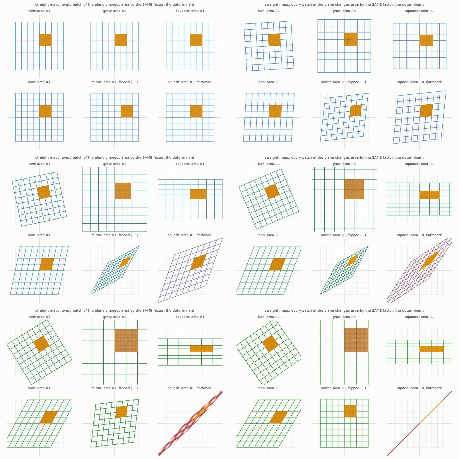
A common pattern appears. Each straight map multiplies the yellow square’s area by a fixed amount. The same multiplier applies to every patch of the plane, wherever that patch begins.
- turn, squeeze, and lean each leave area multiplied by 1
- grow doubles lengths in both directions, so area is multiplied by 4
- mirror keeps the area size the same but reverses the side facing us
- squash multiplies area by 0 and sends the whole plane onto one line
This fixed number is the map’s determinant. Its size records the area multiplier. Its sign records whether orientation was reversed: the mirror has determinant −1 rather than 1. In that way, one number carries both pieces of information.
The crucial case is a determinant of zero.
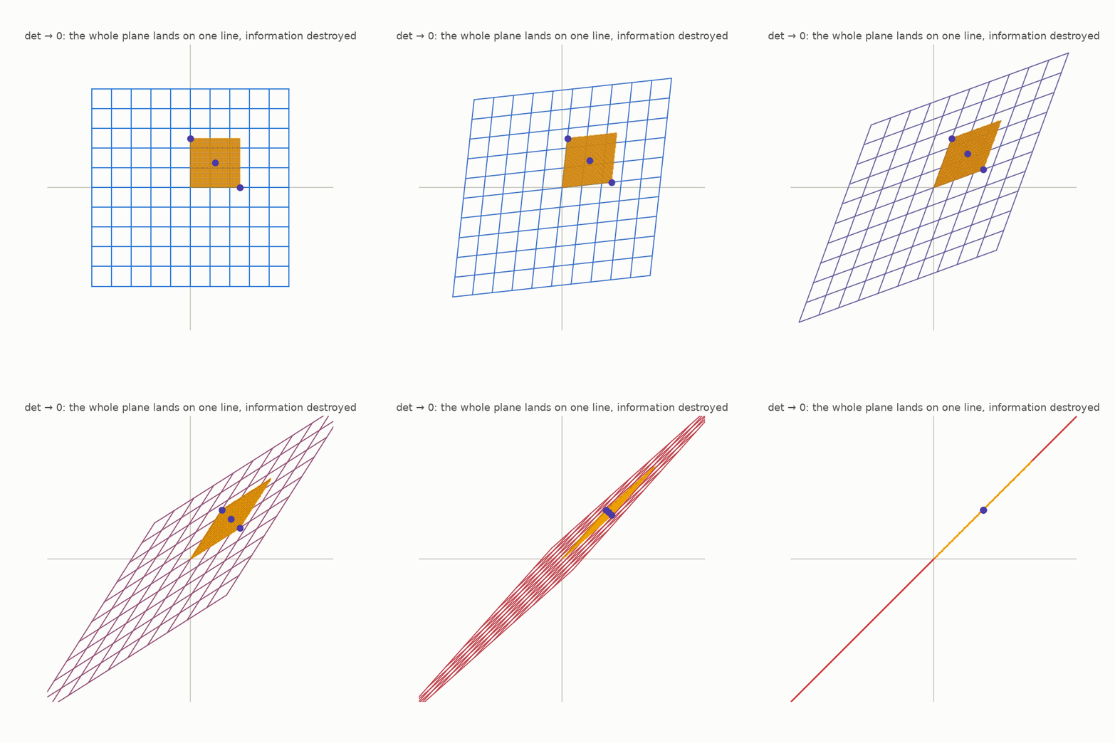
As the figure shows, a zero determinant flattens the plane onto a line. Points that began in different places can then arrive together. Those collisions erase information, so an inverse cannot exist.
When the determinant is not zero, a straight map neither creates collisions nor leaves gaps. It has an inverse, and that inverse is another straight map. For this particular kind of map, the determinant gives a complete test:
A straight map can be undone exactly when its determinant is not zero.
(A straight map is described by four numbers: $F(x, y) = (ax + by,\; cx + dy)$. Its determinant is $ad - bc$. We will use the meaning of this number rather than calculate it by hand.)
Keep in mind: the determinant is the fixed area factor of a straight map. A nonzero determinant allows an inverse; a zero determinant flattens the plane and loses information.
6 · Bending the grid
Polynomial maps can bend a grid as well as move it straight. We will compare maps with an explicit reverse against maps that flatten some area to zero. The distinction leads directly to Keller’s question.
Begin with a map called a shear:
$$ F(x, y) = (x + y^2,\; y) $$This rule slides every horizontal row to the right by an amount determined by $y^2$. Rows near the middle move only a little, while rows farther away move more. The yellow square makes the change in area visible.
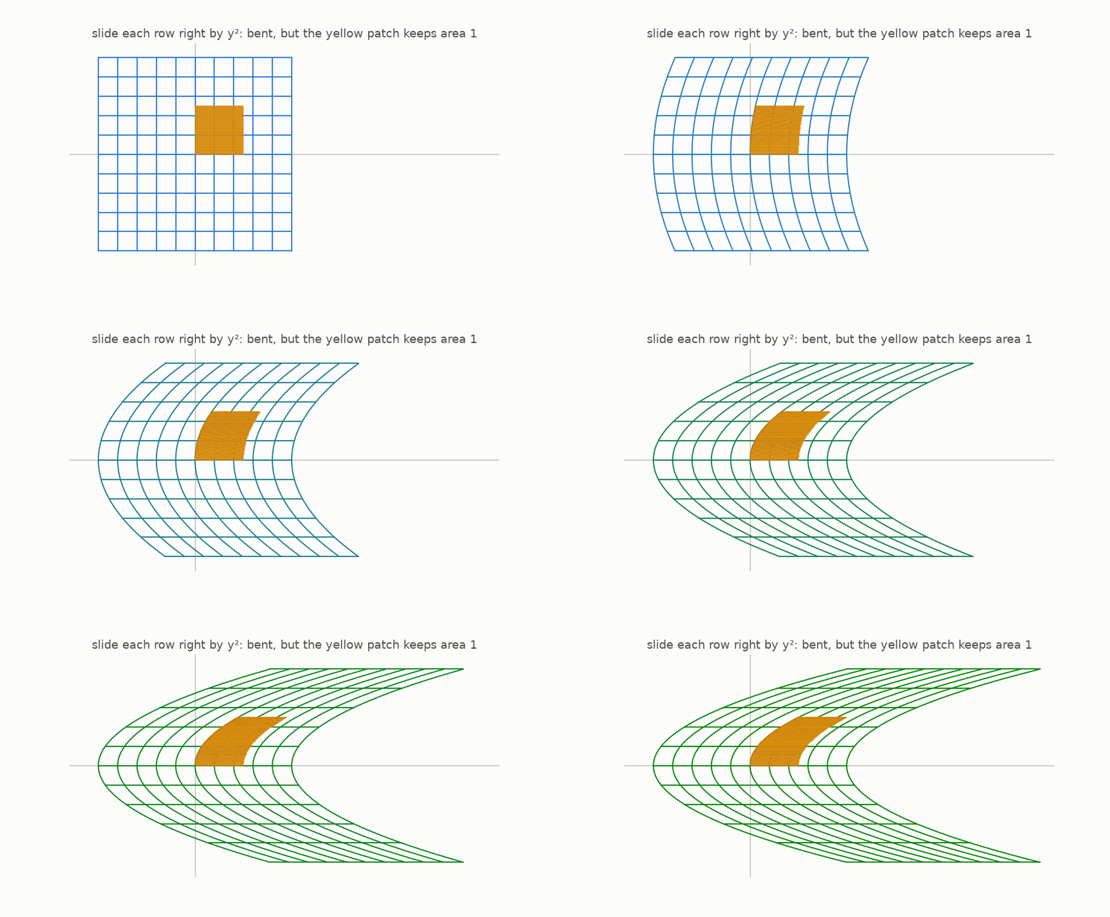
The shape of the yellow patch changes, but its area does not. Every small patch keeps exactly the same area. Reversing the map is straightforward: each row moved right by $y^2$, so the undo rule moves it left by the same amount:
$$ G(x, y) = (x - y^2,\; y) $$Applying $G$ after $F$ returns every point to its starting place. Since $G$ is also polynomial, this gives a non-straight polynomial map with a polynomial inverse.
Several shears may be composed to produce a more complicated map. Apply a vertical shear and then a horizontal one, and the pair becomes this single polynomial map:
$$ H(x, y) = \left(\,x + (y + x^2)^2,\; y + x^2\,\right) $$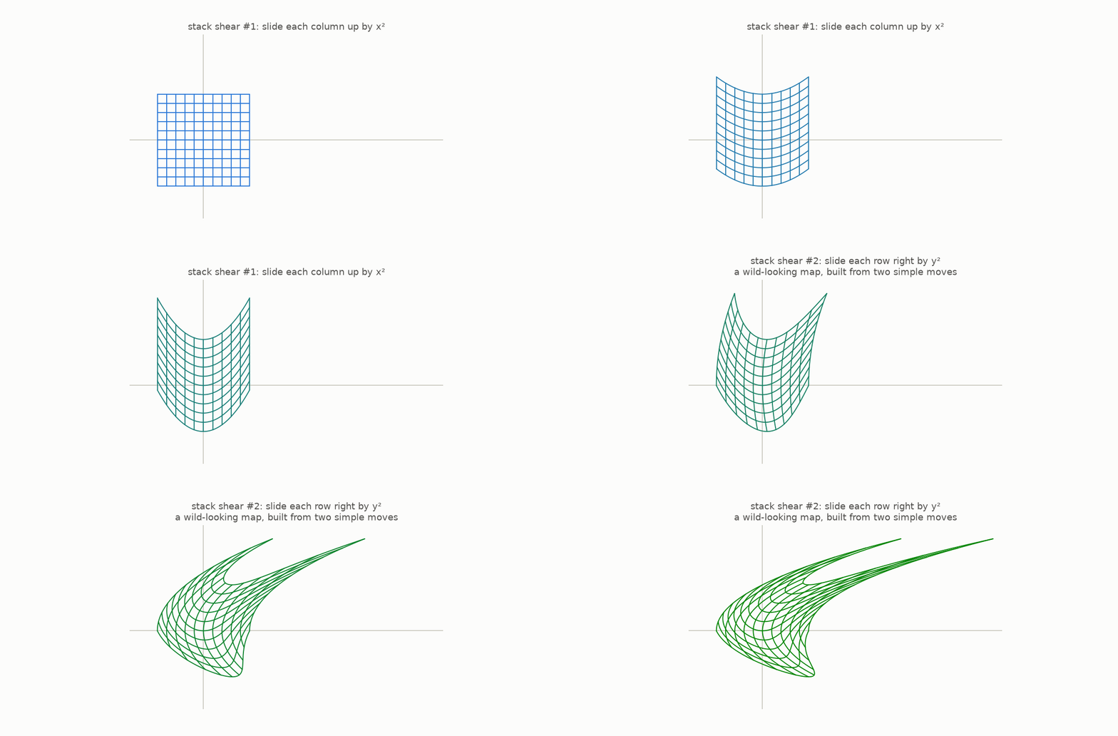
This is the map shown in the opening animation. Although the final grid looks complicated, the construction is only two reversible steps. To undo a sequence, reverse the second step first and then the first, just as clothes are removed in the opposite order from which they were put on. Chapter 10 lets the computer write the resulting polynomial inverse.
Any finite stack of these shears and invertible straight maps remains invertible, because each individual step can be reversed in the opposite order.
Other polynomial maps do lose information.
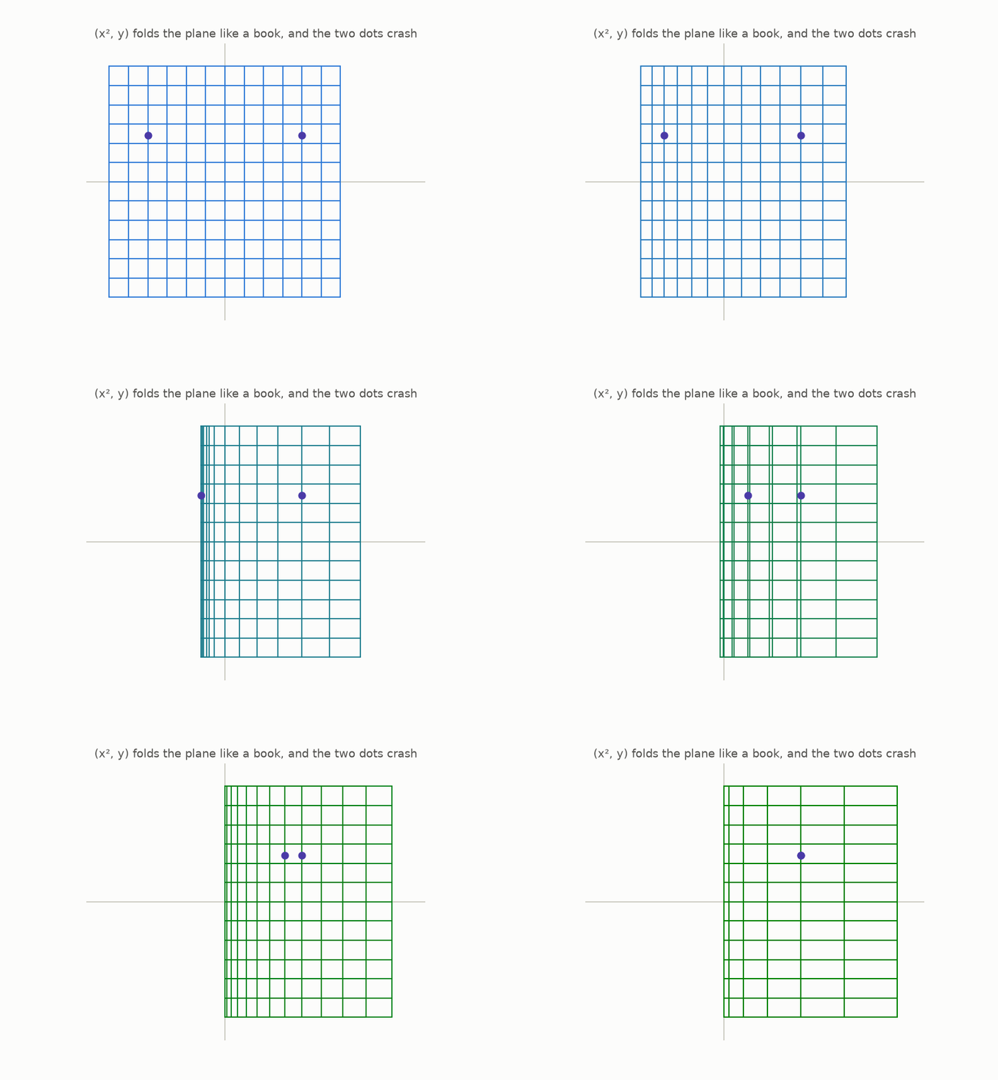
The map $F(x, y) = (x^2, y)$ folds the left half of the plane onto the right half, like closing a book. The marked dots begin at different points but share a destination. Because of that collision, this map has no inverse.
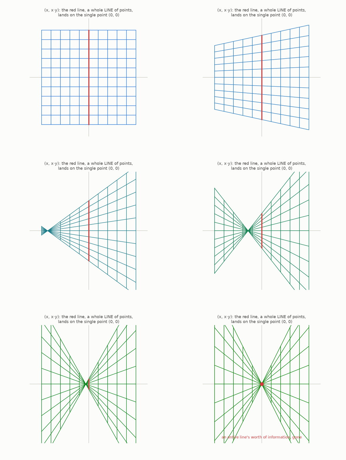
The map $F(x, y) = (x, x\cdot y)$ crushes the entire vertical center line into one point. It also has many inputs with the same output, so it cannot be reversed.
The shears are invertible because their construction supplies a polynomial reverse for every step. The fold and crush are not invertible because they flatten area to zero and create collisions.
For straight maps, chapter 5 said that a nonzero area factor is exactly what permits an inverse. A bent map has no single area multiplier for the whole plane; it may stretch area differently at different locations. To measure what happens at one location at a time, we need a microscope.
Keep in mind: compositions of reversible shears can bend the plane dramatically and still be undone. A fold or crush creates collisions by flattening area, so no inverse is possible.
7 · The microscope
The next term is Jacobian. Its role is easier to understand by thinking of a microscope that shows what a map does near one chosen point.
First, zoom in on one point of the curved graph $y = x^2$.
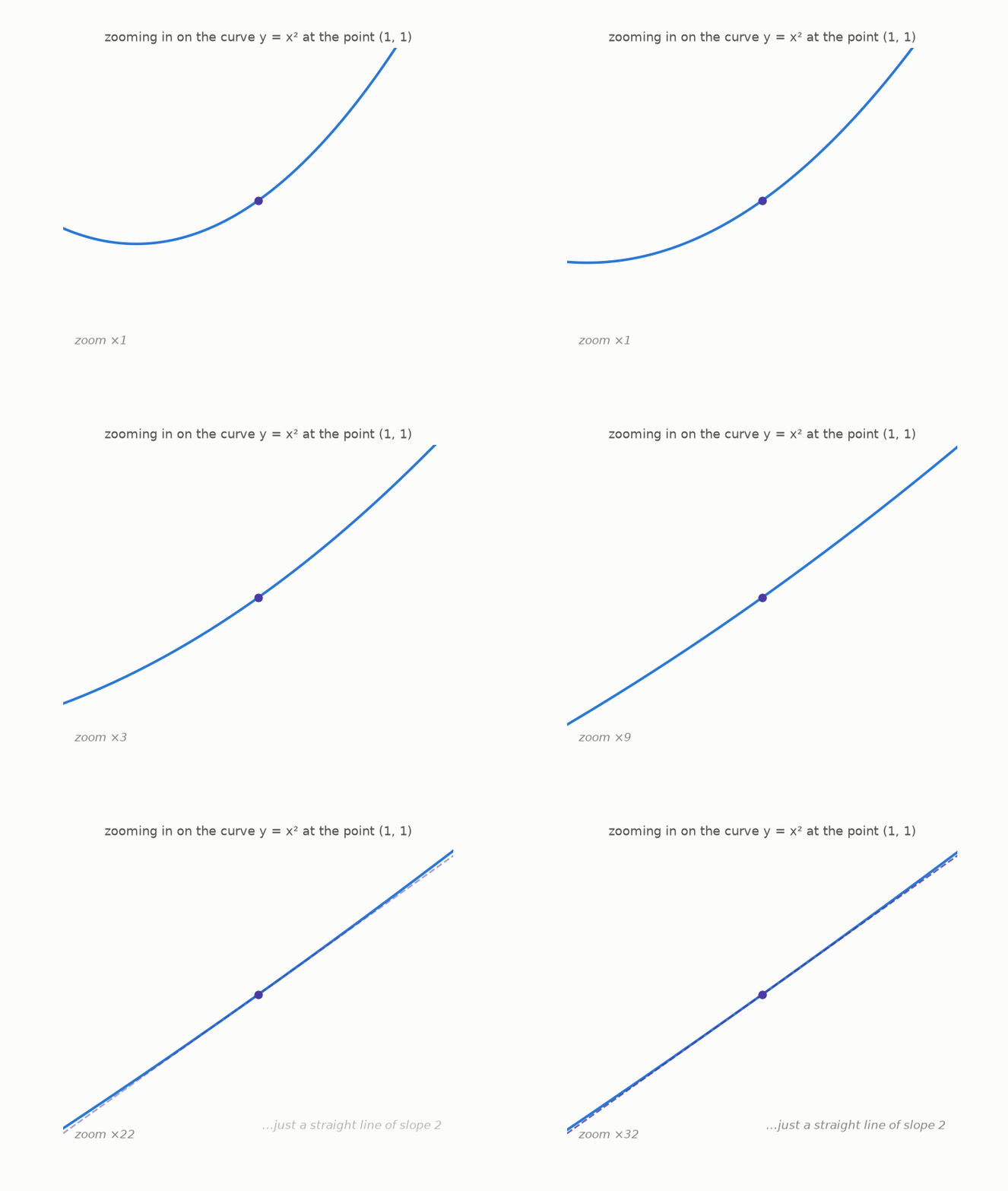
As the view gets closer, the curve looks more and more like a straight line. The slope of that limiting line, which is 2 at the point shown, is called the derivative there. For this article, the needed idea from calculus is simply that a smooth curve looks straight when viewed closely enough.
The same zoom can be applied to a bent grid. Take the stacked-shear map $H$ from chapter 6, choose the point $p = (0.5,\, 0.5)$, and inspect what the map does close to that point.
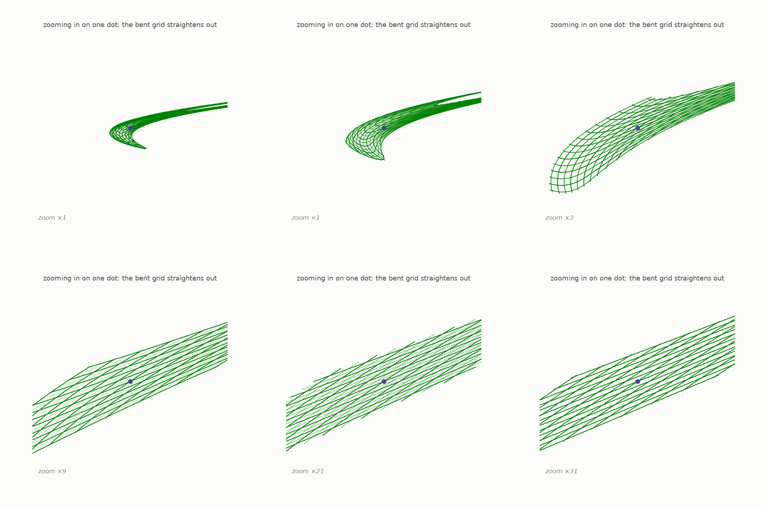
The nearby grid increasingly resembles straight, parallel, evenly spaced lines—the kind of picture used in chapter 5. At very small scales, a bent polynomial map is approximated by a straight map.
The Jacobian of $F$ at a point $p$ is the straight map that describes this close-up behavior near $p$.
The close-up may differ from one point to another, so the Jacobian depends on where the microscope is placed. A computer obtains it through a standard table of derivatives. We will not calculate that table by hand; chapter 10 uses the computer to do it.
This matters because every straight map has a determinant. At each point $p$, the determinant of the local straight map gives a local area factor, written $\det J_F(p)$. It describes how the map changes a tiny patch near that point and whether the close-up reverses its orientation.
The next figure colors the plane according to this local factor for two maps. A moving probe samples the value at its current position.
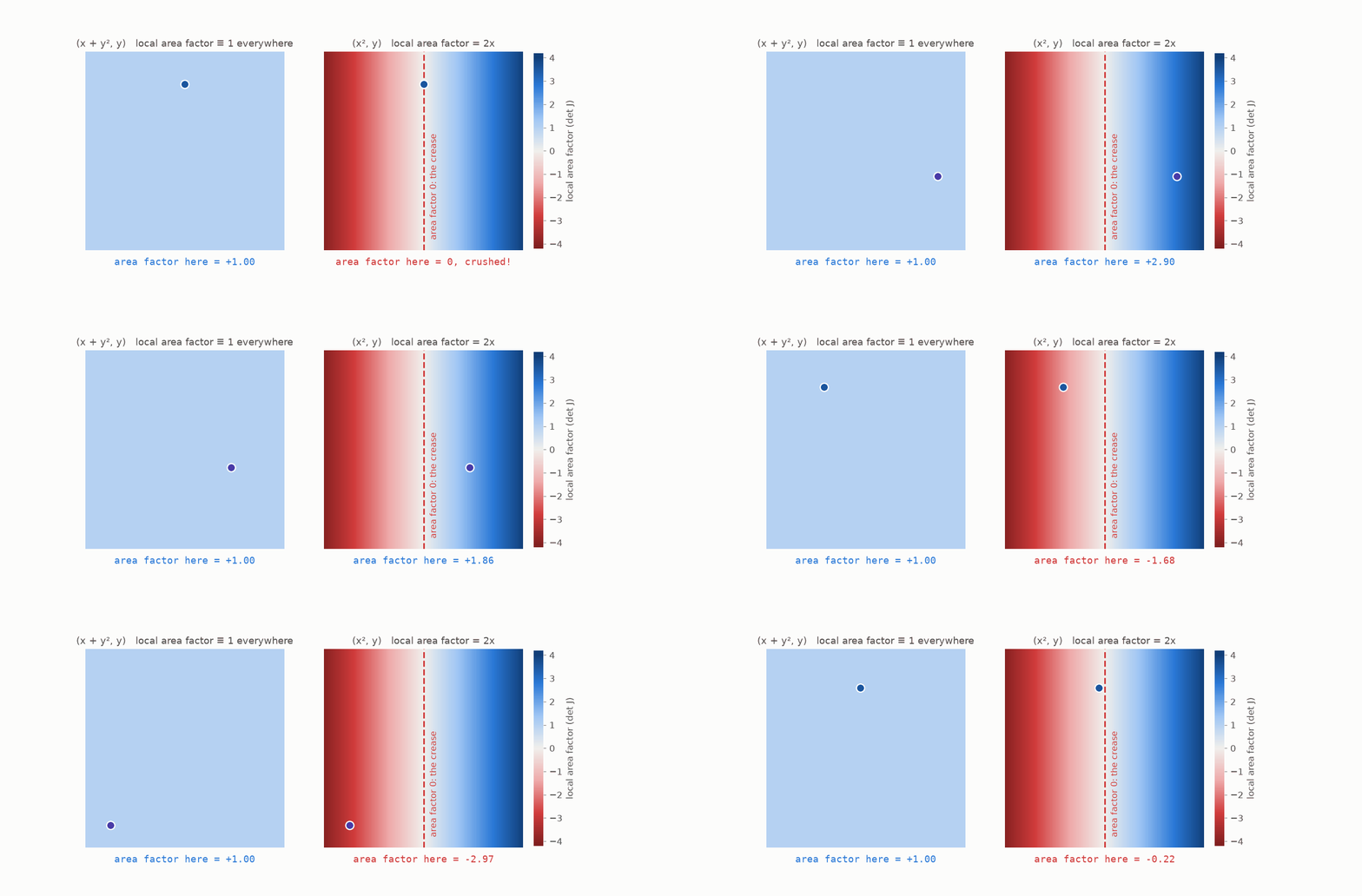
- For the shear $(x + y^2, y)$, the local area factor is 1 at every point. Wherever the microscope is placed, its straight-map approximation preserves area.
- For the fold $(x^2, y)$, the local area factor is $2x$. It is positive on the blue right half, negative on the red left half where orientation is reversed, and zero along the fold line. The zero line is where the close-up becomes flat.
Keep in mind: the Jacobian is the straight map seen in a close-up around one point. Its determinant is the local area factor; when that number is zero, the close-up has a flattened direction.
8 · Local vs global
The microscope gives detailed information near one point, but it cannot see the whole map at once. A map may behave well in every small neighborhood being inspected while distant parts of the space still meet.
This suggests a tempting test: check the local area factor at every point. If that factor never vanishes, no tiny neighborhood is flattened. It is natural to ask whether this already guarantees a global inverse.
One part of the idea is correct. If the local factor at a point $p$ is nonzero, the map has an inverse in some sufficiently small neighborhood of $p$. This is the inverse function theorem. Its promise is local, not global.
The following example shows the difference between those two scales.
Apply the polynomial map $F(x, y) = (x^2 - y^2,\; 2xy)$ to a ring around the center. In the picture, the right half is blue and the left half is gold.
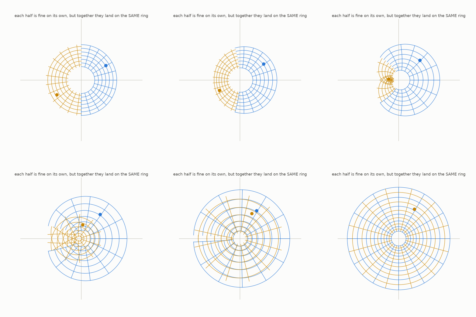
Every point on that ring has a healthy close-up: there is no crease or flattening nearby. Nevertheless, the blue half covers the entire target ring, and the gold half covers the same target ring again. Each target point has two starting points, one on each side. The blue and gold dots make one such collision visible.
The colliding inputs are far apart. A microscope centered on either one cannot include the other, so it reports no local problem. The map works locally around those points but fails as a single global undoable map.
Across the full plane, the local area factor for this map is $4(x^2 + y^2)$.
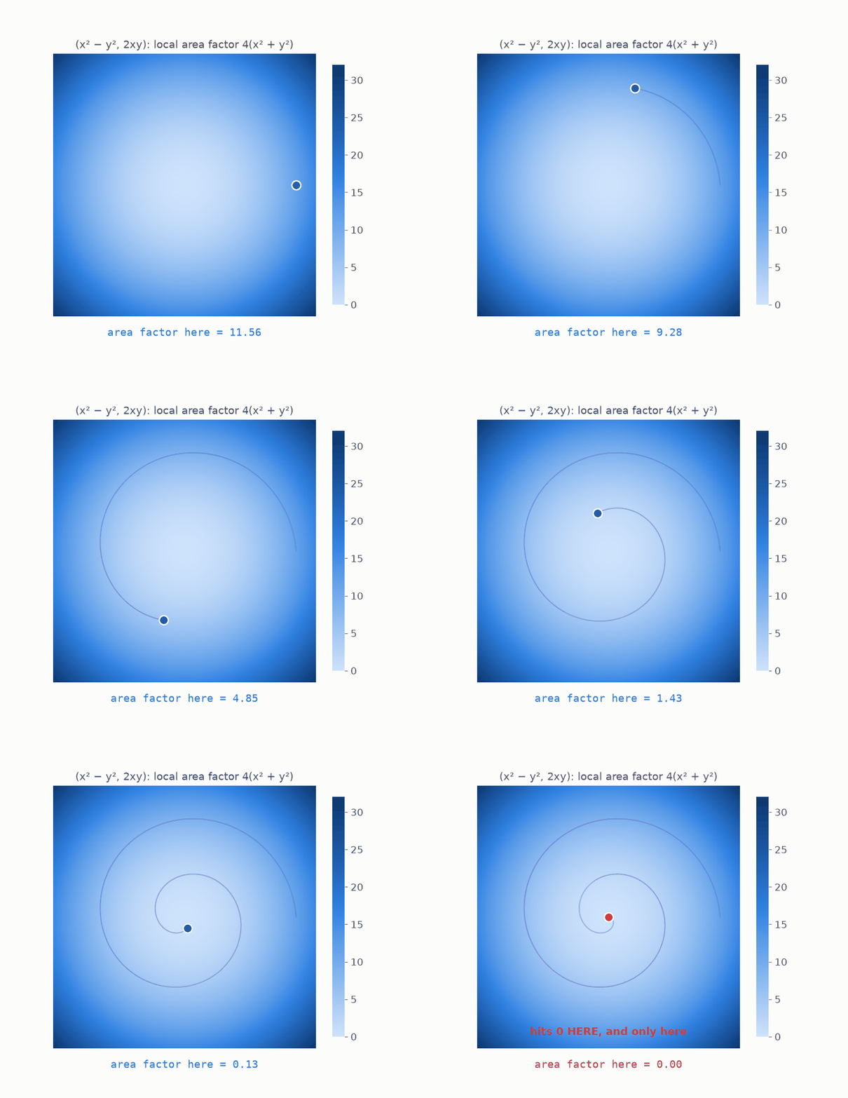
This factor is zero only at the center and positive everywhere else. Thus the full map has just one point where the local test fails, yet it still covers most outputs twice.
This example must be interpreted carefully. Because its factor does reach zero at the center, it does not disprove the proposed “nonzero everywhere” test. It shows a different danger: a collision may join distant inputs that cannot be viewed through one local microscope. Local information and global undoability answer different questions.
Could the test work if the local factor were nonzero with no exceptions? Over the real numbers, it still does not. Chapter 11 describes Pinchuk’s polynomial map, whose factor is positive at every real point even though two distant inputs collide. Smooth non-polynomial maps can behave more extremely and hit some outputs infinitely many times.
A merely nonzero local factor is therefore insufficient over the real numbers. Keller imposed a tighter condition for polynomial maps over the complex numbers: the local factor must be the same nonzero constant at every point. The question was whether those requirements finally force a global polynomial inverse.
That question is the Jacobian Conjecture, stated in full in the next chapter.
Keep in mind: the Jacobian describes one small neighborhood at a time. Inputs far apart can still collide, so local invertibility does not by itself provide a global inverse.
9 · The conjecture
We can now collect the pieces:
- Undoable means that there are no collisions and no gaps (chapter 2).
- Polynomial maps have coordinate rules built from addition and multiplication (chapters 3 and 4).
- Determinant is the area factor of a straight map, with zero indicating a flattened direction (chapter 5).
- Jacobian is the local straight-map approximation, and $\det J$ is its local area factor (chapter 7).
- The difficulty is that good local behavior does not automatically control collisions between distant points (chapter 8).
Keller’s 1939 question strengthens the local requirement. Instead of asking only that the factor avoid zero, require it to have one fixed nonzero value at every point. The shear and stacked shears have value 1 everywhere. Keller also restricted the rules to polynomials.
He asked whether every map meeting those conditions must have a polynomial inverse.
The Jacobian Conjecture (Keller, 1939)
Take any polynomial map, in any dimension.
Suppose its local area factor is the same nonzero constant at every point.
Then the map can be undone, and its undo is also a polynomial map.
The animation below presents the condition first and then asks whether the motion must always be reversible.
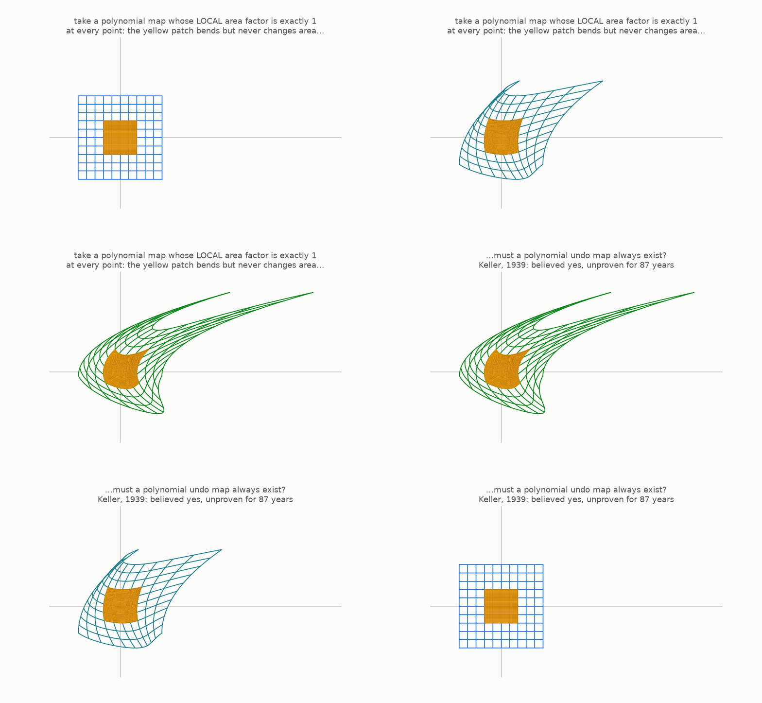
This was known as the Jacobian Conjecture. Calling it a conjecture meant that it was expected to be true but had not been proved.
Three details complete the statement:
- All dimensions. The question applies to the plane, to three-dimensional space, to four-dimensional space, and onward. In each case, every output coordinate is a polynomial in all the input coordinates. Most pictures here use two dimensions because a flat grid is easier to view.
- Complex numbers. The official conjecture is set over the complex numbers. In that number system, a polynomial local factor that never equals zero must be a nonzero constant. The two conditions are not equivalent over ordinary real numbers, and chapter 11 gives a real counterexample. The choice of number system is therefore essential.
- Only collisions matter. The Ax–Grothendieck theorem says that an injective complex polynomial map is automatically surjective and has a polynomial inverse. In the language of chapter 2, once collisions are ruled out, gaps and the form of the inverse take care of themselves.
Every qualifying map shown so far has factor 1 and an explicit inverse. Further calculations and several theorems also supported the conjecture, including a proof for all maps of degree at most 2. By the end of the twentieth century, there was substantial evidence in its favor.
Still, no proof covered the full statement between 1939 and 2026.
Keep in mind: the Jacobian Conjecture asked whether a polynomial map with one fixed nonzero local factor must have a polynomial inverse.
10 · Test it yourself
Before turning to the eventual counterexample, we can test the conjecture on the stacked-shear map using exact computer algebra rather than numerical estimates.
Python’s sympy library manipulates polynomials symbolically, much as a long pencil-and-paper calculation would. The companion repository provides a few helper functions. This session uses the map $H(x,y) = (x + (y+x^2)^2,\; y + x^2)$:
>>> from jacobian_guide.core import jacobian_det, invert, compose, degree
>>> from jacobian_guide.examples import VARS, TANGLED   # TANGLED is H

>>> jacobian_det(TANGLED, VARS)          # local area factor, symbolically
1
The result is the constant 1. Because the program simplified the polynomial formula itself, this check covers all input points at once rather than a sample of points. Thus $H$ meets Keller’s condition. We can then ask the program for its inverse:
>>> G = invert(TANGLED, VARS)
>>> G
(x - y**2, -x**2 + 2*x*y**2 - y**4 + y)

>>> compose(G, TANGLED, VARS)            # undo after do = ?
(x, y)
The returned inverse is another polynomial. Composing it with $H$ simplifies to $(x, y)$, which leaves every input unchanged. This confirms symbolically that each point returns to its original position.
The fold $(x^2, y)$ provides a useful comparison. Its local area factor is $2x$, not a constant, so it does not meet the conjecture’s condition. Its failure to have an inverse neither supports nor contradicts the conjecture.
The following table summarizes the examples tested in the repository:
| map | local area factor | undoable? | degree, undo degree |
|---|---|---|---|
| shear $(x+y^2,\,y)$ | 1 | yes | 2, 2 |
| stacked map $H$ | 1 | yes | 4, 4 |
| triple-stacked $H_3$ | 1 | yes | 4, 4 |
| fold $(x^2,\,y)$ | $2x$, does not qualify | no | n/a |
All three qualifying examples in the table agree with the conjecture. Earlier theory supplied stronger evidence:
- Degree at most 2 was proved (Wang, 1980): in any dimension, every map of degree 2 or less that satisfies the condition has a polynomial inverse.
- Degree 3 contains the full problem (Bass–Connell–Wright, 1982): proving the conjecture for all degree-3 maps would prove it for every degree. Even after this reduction, the general case remained unresolved.
- The plane was checked through degree 100 (Moh, 1983, with computer assistance).
There is an important difference between dimensions. For invertible polynomial maps of the plane, the inverse has the same degree as the original map. In dimensions three and higher, the inverse can have much larger degree. This was one indication that higher-dimensional behavior might be less controlled.
Keep in mind: the examples above support the conjecture, degree 2 was settled, and a reduction showed that degree 3 already contained the general difficulty.
11 · Why it was so hard
The successful tests did not remove several basic obstacles. Any general proof had to handle the number system, the behavior far from the center of the space, and the difference between local and global information. These issues exposed errors in a long series of proposed proofs.
This is the most demanding chapter, but it uses only ideas already introduced: functions, inverses, collisions, polynomials, and local area factors. Each obstacle begins with a plausible proof strategy and then gives an example showing why that strategy alone cannot work.
1884       Kraus claims a proof. It leaks at infinity.
1939       Keller poses the conjecture.
1955-61    A wave of published proofs. All wrong.
1980       Wang: true for degree 2 and below.
1982       Bass, Connell, Wright: degree 3 decides everything.
1983       Moh: true in the plane up to degree 100.
1994       Pinchuk: the real-number version is false.
1998       Smale lists it as Problem 16 for the new century.
2004       Nagata's map proved wild. 3D is stranger than the plane.
2026       Counterexample. False in dimension 3 and up. Plane still open.
The historical pattern repeated many times: a proof was announced, examined, and eventually found to have a gap. Examples include Kraus in 1884, before Keller’s formulation, Engel in 1955, three attempts by Segre, Gröbner’s attempt, and later submissions.
Obstacle 1: the statement is false over the real numbers.
The proposed route: all the pictures so far use the ordinary real plane. Perhaps real geometry is enough, and a real polynomial map with a local area factor that never vanishes must always be invertible.
Why it fails: in 1994, Sergey Pinchuk constructed two explicit polynomials of degrees 10 and 25. Their local area factor is positive at every real point, but the resulting map still sends different inputs to the same output. The animation samples this positive factor along the probe’s path; an exact argument proves that it never reaches zero anywhere on the real plane.
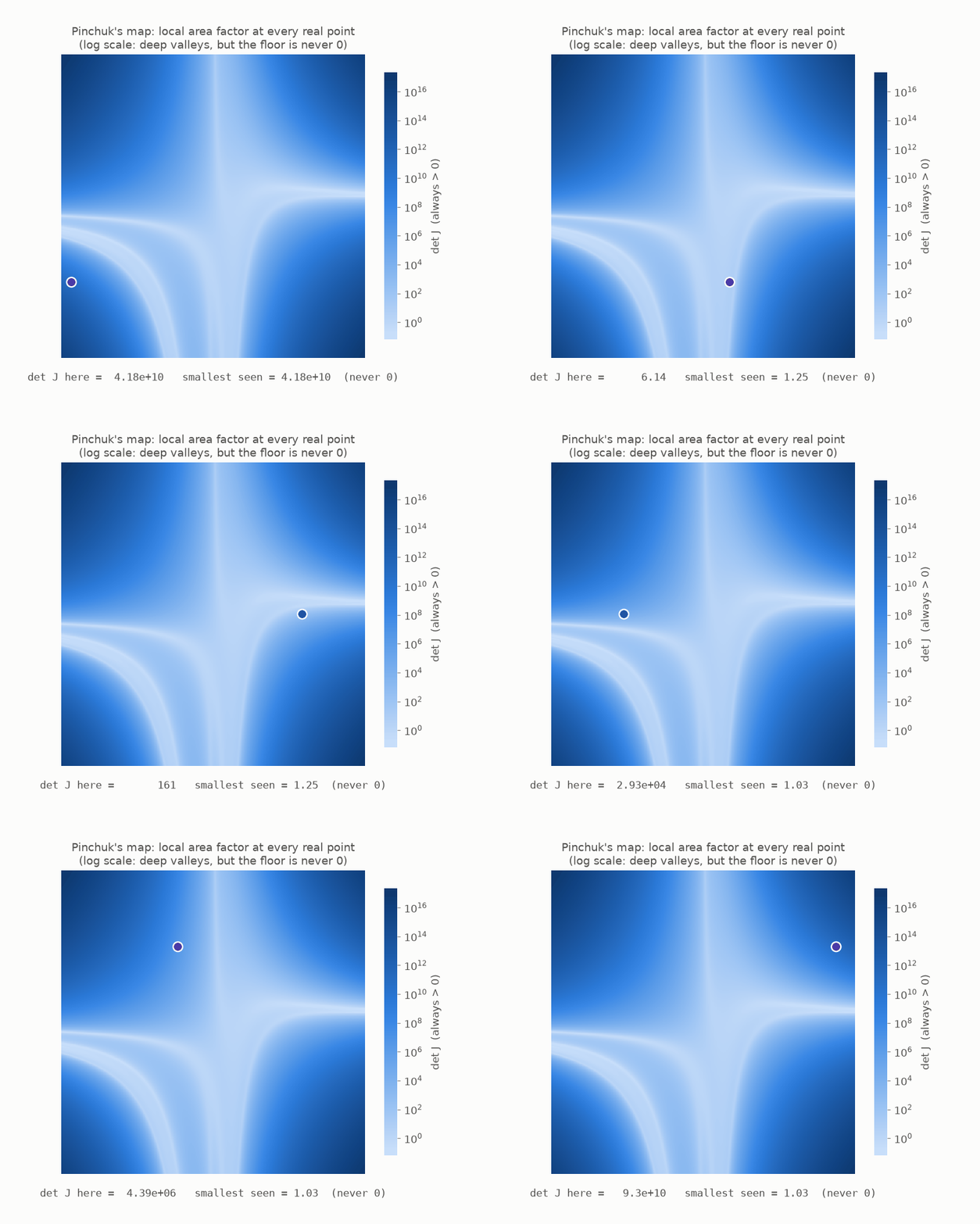
Pinchuk’s map has no local flattening and no local orientation reversal, yet it has a global collision. It supplies the example promised in chapter 8 and shows that the corresponding statement over real numbers is false.
This raises an obvious question: why does Pinchuk’s example not disprove the official conjecture? The official problem uses complex numbers, and the feature that protects Pinchuk’s factor over the reals does not carry over. Over real numbers, squares are never negative, so a sum of squares can stay positive. Complex numbers are not ordered into positive and negative values in this way. Over the complex numbers, a polynomial in several variables with no zeros must be constant. Pinchuk’s factor is not constant, so it has complex zeros and does not meet Keller’s condition there.
(More specifically, Pinchuk’s factor is $t^2 + \big(t + f\,(13 + 15h)\big)^2 + f^2$ for certain helper polynomials $t, f, h$. Over the reals this is a sum of three squares, and a short additional argument proves it is never zero. The symbolic identity is checked in tests/test_pinchuk.py.)
Obstacle 2: the statement is false in clock arithmetic.
The proposed route: since polynomials are symbolic expressions, perhaps a proof can rely only on algebraic manipulations that work in every number system.
Why it fails: consider clock arithmetic, in which values wrap around after a fixed number of positions. On a clock with a prime number $p$ of positions, the rule $F(x) = x - x^p$ has constant slope 1. Even so, it sends every clock position to 0, producing a complete collision.
The next animation shows this on a clock with 5 positions.
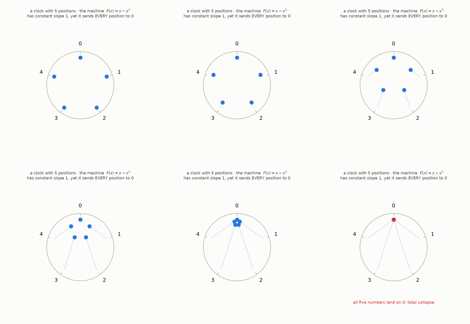
Thus the analogous conjecture fails in clock arithmetic. A valid proof over the complex numbers would have to use a property that ordinary and complex numbers possess but clock arithmetic lacks. The standard name for that property is characteristic zero. Symbolic steps valid in every number system cannot be sufficient by themselves.
Obstacle 3: the danger sits at infinity.
The proposed route: Hadamard’s theorem says that a map which is locally invertible everywhere and does not allow inputs to escape to infinity while their outputs stay bounded is globally invertible. Perhaps polynomial maps automatically prevent that kind of escape.
Why that route needs more: polynomial maps can exhibit exactly this behavior. The crush map $(x, xy)$ does not satisfy Keller’s condition, so it is not itself a counterexample. It does show that being polynomial alone offers no protection. The inputs $(\tfrac12, 2), (\tfrac13, 3), (\tfrac14, 4), \dots$ travel farther and farther away, while their outputs $(\tfrac12, 1), (\tfrac13, 1), (\tfrac14, 1), \dots$ approach the ordinary point $(0, 1)$.
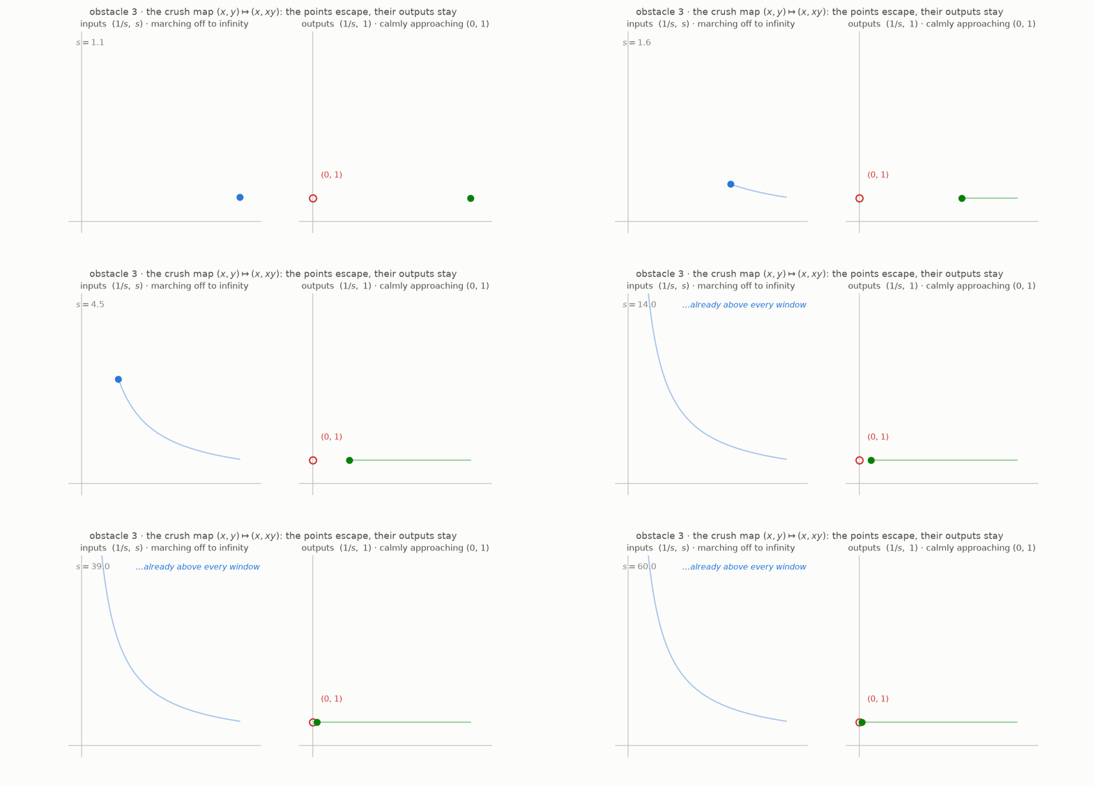
A proof therefore needs genuine control over what happens near infinity; polynomial form alone does not supply it. Faulty control of this region was already the weakness in Kraus’s 1884 argument.
There was also a warning from dimension 3. Every complicated invertible map built earlier in this article was composed from shears and straight maps. Such a composition is automatically invertible. In the plane, every invertible polynomial map can in fact be decomposed this way. Nagata’s three-dimensional map behaves differently: it has local factor 1 and a polynomial inverse, but Shestakov and Umirbaev proved in 2004 that it cannot be assembled from shears and straight maps. This established that three-dimensional polynomial maps include structures absent from the plane.
Keep in mind: a proof had to use the polynomial form, the complex-number setting, and control at infinity together. Pinchuk blocks a real-only argument, clock arithmetic blocks a number-system-independent argument, and polynomial maps can still behave badly near infinity.
12 · The fall
In July 2026, an explicit map settled the conjecture in dimensions three and higher. The two-dimensional case, where Keller’s question began, was not settled.
An explicit counterexample in three variables was announced on July 19–20, 2026. The construction was credited to mathematician Levent Alpöge, in response to a version of the question raised by a colleague, and the final example was produced with help from the AI model Claude Fable. No peer-reviewed paper was available when this article was written, so the attribution and surrounding account should be treated as provisional. The algebraic claims themselves are independently checked with exact arithmetic in tests/test_counterexample.py.
The map. Use $u = 1 + xy$ as an abbreviation. It sends a point $(x, y, z)$ in three-dimensional space to another point $(P, Q, R)$:
$$ \begin{aligned} P &= u^3\,z + y^2\,u\,(4 + 3xy) \\ Q &= y + 3x\,u^2\,z + 3xy^2\,(4 + 3xy) \\ R &= 2x - 3x^2 y - x^3 z \end{aligned} $$The three components are polynomials of degrees 7, 6, and 4, with small integer coefficients.
Fact 1: the condition holds. The local volume factor—the three-dimensional Jacobian determinant—is the constant $-2$ at every point. This meets Keller’s condition. The minus sign records a uniform reversal of orientation; the size of the factor remains fixed.
Fact 2: the map has a collision. These three different inputs all have the same output:
(  0,     0,  -1/4 )   →   ( -1/4, 0, 0 )
(  1,  -3/2,  13/2 )   →   ( -1/4, 0, 0 )
( -1,   3/2,  13/2 )   →   ( -1/4, 0, 0 )
The three-dimensional animation traces each input to its image. All three paths finish at the same red X.
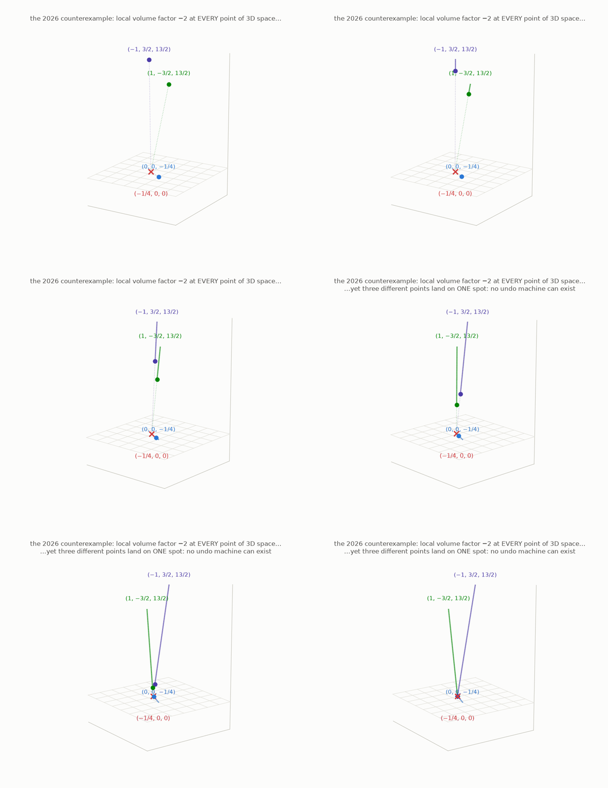
At the output $(-\tfrac14, 0, 0)$, there is no unique way to recover the input because three starting points lead there. This is exactly the kind of collision introduced in chapter 2. It proves that the Jacobian Conjecture is false in three dimensions.
The same counterexample extends to every higher dimension. In four dimensions, leave the extra coordinate unchanged: $(x,y,z,w) \mapsto (P, Q, R, w)$. The local volume factor remains $-2$, and the original three inputs still collide. Additional unchanged coordinates give the same result in dimensions 5, 6, and above.
A direct arithmetic check. Begin with the third output, $R = 2x - 3x^2y - x^3z$, and substitute the three points:
- $(0,\ 0,\ -\tfrac14)$: $\quad R = 0 - 0 - 0 = 0$ ✓
- $(1,\ -\tfrac32,\ \tfrac{13}{2})$: $\quad R = 2 - 3\cdot(-\tfrac32) - \tfrac{13}{2} = 2 + \tfrac92 - \tfrac{13}{2} = 0$ ✓
- $(-1,\ \tfrac32,\ \tfrac{13}{2})$: $\quad R = -2 - \tfrac92 + \tfrac{13}{2} = 0$ ✓ (Here $-3x^2y = -\tfrac92$, while $-x^3z = +\tfrac{13}{2}$ because $x^3 = -1$.)
For the first input, the other two outputs are also short to check. At $(0, 0, -\tfrac14)$, the abbreviation $u$ equals 1. It follows that $P = 1 \cdot (-\tfrac14) + 0 = -\tfrac14$ and $Q = 0 + 0 + 0 = 0$. This confirms that the first point maps to $(-\tfrac14, 0, 0)$.
An exact computer check. Substituting the other two inputs by hand requires more fraction arithmetic. The following code checks all three images and the constant volume factor exactly:
from sympy import symbols, Matrix, Rational

x, y, z = symbols("x y z")
u = 1 + x*y
P = u**3*z + y**2*u*(4 + 3*x*y)
Q = y + 3*x*u**2*z + 3*x*y**2*(4 + 3*x*y)
R = 2*x - 3*x**2*y - x**3*z

print(Matrix([P, Q, R]).jacobian([x, y, z]).det().expand())   # -> -2

for pt in [(0, 0, Rational(-1, 4)),
           (1, Rational(-3, 2), Rational(13, 2)),
           (-1, Rational(3, 2), Rational(13, 2))]:
    print([f.subs(dict(zip((x, y, z), pt))) for f in (P, Q, R)])
# -> [-1/4, 0, 0]  three times
The repository provides the same verification as a test: python -m pytest tests/test_counterexample.py -q.
What remains open. Keller’s original 1939 question concerned the plane. The counterexample above uses three variables and does not settle the two-variable case. Earlier warning signs also separate these dimensions: wild invertible maps occur from dimension 3 onward, and inverse degrees can grow much more sharply there. The plane case has been verified through degree 100 but remains open.
What the result changes. The long-standing expectation was that “polynomial map plus constant local factor” should force a global polynomial inverse. The three-dimensional map shows that these conditions are not sufficient. Its behavior also confirms that control at infinity was a real obstruction rather than a technical nuisance: a degree-7 polynomial map can exploit it while maintaining a constant Jacobian determinant.
The arithmetic and code above verify the two decisive properties: the determinant is constant, and distinct inputs share an output.
Keep in mind: an explicit degree-7 map of three-dimensional space has constant volume factor $-2$, yet three different points share one output. The Jacobian Conjecture is therefore false in dimensions 3 and higher and still open in the plane.
Where to go next
- The companion repository, github.com/muchmirul/conjectures, contains the figure code, exact-algebra helpers, tests, and research notes with sources.
- A. van den Essen, Polynomial Automorphisms and the Jacobian Conjecture, is a standard advanced reference.
- T. Tao’s blog post on the Ax–Grothendieck theorem explains why “no collisions” implies “no gaps” in this setting.
- L. A. Campbell, Picturing Pinchuk’s Plane Polynomial Pair (arXiv:math/9812032), treats the real counterexample visually.
- The Wikipedia article Jacobian conjecture provides current status and further references.