Condensed mathematics, part 3 of 3

Measure Rules for Rings and Geometry

This is the third and final part on condensed mathematics. Part two gave abelian groups a rule for integrating integer-valued measures. Different rings need different rules, especially the real numbers. We will let each ring carry a suitable theory of measures, then use the resulting framework to build compactly supported cohomology, the six operations, and coherent duality. Parts one and two are assumed.

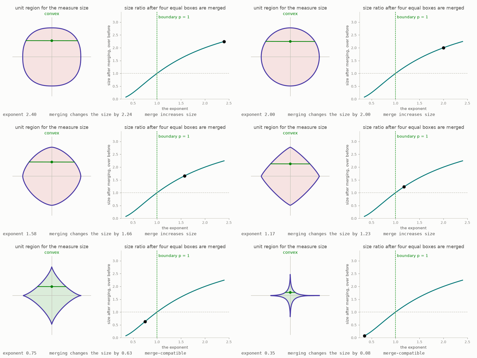
As an exponent decreases, a rounded unit region becomes a diamond and then bends inward

The animation previews the main example. Each shape contains the pairs of weights whose size is at most one. An exponent controls the shape. Above one, the region is rounded and convex. At one, it is a diamond. Below one, it bends inward and is no longer convex. A separate calculation shows that merging boxes preserves the size limit only when the exponent is at most one. The real theory must therefore work at and below the point where ordinary local convexity stops applying.

This part covers Lectures VII to XI of Peter Scholze's Lectures on Condensed Mathematics (arXiv:2605.03658, May 2026), which present joint work with Dustin Clausen. Part one introduced probes and condensed sets. Part two developed compatible integer measures and solid groups. Each chapter below includes a finite activity, but the categorical theorems are quoted from the lectures. The part-three activity list links to all nine pages.

    choose a measure rule        1  a ring and its legal measures
                                2  p-adic and discrete examples
                                3  the rule needed by the real numbers
    build local geometry         4  global functions and boundary tails
                                5  compactly supported cohomology
                                6  gluing affine patches
    organize the result          7  the six operations
                                8  coherent duality

Use the controls to change the picture. Open the activity on its own page

1 · A ring and its legal measures

Part two used one fixed summation rule based on integer-valued measures. That rule does not suit every ring. The real numbers and the $p$-adic numbers have different ideas of convergence, so they should not be forced to use the same completion.

A ring has addition, subtraction, and multiplication. A module is an additive group whose elements can also be multiplied by elements of the ring. For each probe, we want to specify which weighted combinations of its points are allowed in a module and how those combinations behave.

The general definition has two pieces (Definition 7.1, page 45). First, we choose a condensed ring $A$. As in part one, its probe values contain topological information together with algebraic operations. Second, for every extremally disconnected probe $S$, we choose an $A$-module $\mathcal M[S]$ of allowed measures.

The measure modules must include all Dirac measures, which place unit weight at one point. They must also respect finite disjoint unions. Measures on two separate probes should be the same as one independent measure on each probe.

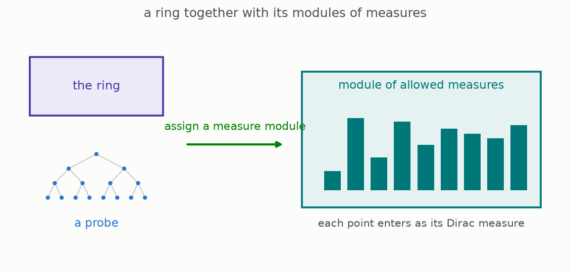
A probe maps to its module of allowed measures, and every point enters as a Dirac measure

These visible rules are necessary but not sufficient. The proposed measure theory must remain stable when its modules are used in exact sequences and chain complexes. Definition 7.4, page 46 gives the derived compatibility test. A pair that passes it is called an analytic ring.

This distinction matters because a rule can look sensible on each individual probe and still fail after modules are combined. Chapter 3 shows this for several natural real-valued measure rules.

The mathematics

Definition 7.1, page 45 of the lectures defines a theory of measures on a condensed ring $A$ as a functor

$$ \mathcal M:\{\text{extremally disconnected }S\} \longrightarrow A\text{-}\operatorname{Mod}, \qquad S\longmapsto\mathcal M[S], $$

The definition also includes a natural Dirac map $S\to\mathcal M[S]$, which sends each point to its unit measure. For disjoint probes, the measure modules must satisfy

$$ \mathcal M[S_1\sqcup S_2]\cong\mathcal M[S_1]\times\mathcal M[S_2]. $$

Definition 7.4, page 46 calls the pair analytic when, for the specified complexes $C$,

$$ R\!\operatorname{Hom}_A(\mathcal M[S],C) \xrightarrow{\sim} R\!\operatorname{Hom}_A(A[S],C). $$

Reading the symbols. The ring is $A$, and $A$-$\operatorname{Mod}$ is the category of condensed $A$-modules. The functor $\mathcal M$ assigns a module of legal measures $\mathcal M[S]$ to each extremally disconnected probe $S$. The map $S\to\mathcal M[S]$ sends each point to its Dirac measure. The symbol $\sqcup$ means disjoint union, $\times$ means product, and $\cong$ means isomorphic. The notation $A[S]$ is the free $A$-module on the points of $S$. The letter $C$ names a chain complex made from free measure modules. The expression $R\!\operatorname{Hom}_A$ is the derived object of $A$-linear maps. An arrow marked $\sim$ is an isomorphism.

Why it matters. The first two displays describe a proposed summation rule. The final isomorphism tests whether that rule survives the homological constructions used later. Passing the finite rules alone does not prove that a pair is analytic.

In the simulation. Choose a ring $A$ and a proposed module $\mathcal M[S]$. Two controls check whether point masses are included and whether disjoint pieces give a product. The final result represents the additional analytic condition as a quoted fact rather than treating the finite checks as a proof.

Use the controls to change the picture. Open the activity on its own page

2 · Two analytic examples

The first examples extend the solid measures from part two. They use the same general definition with two different coefficient rings.

For the $p$-adic rule, use the $p$-adic integers as the ring. On every probe, take compatible measures with values in the $p$-adic integers. Proposition 7.8, page 48 proves that this pair is analytic, so $p$-adic summation fits the general framework.

For the solid rule over a discrete ring, let $A$ be any ring with the discrete topology. Begin with compatible integer measures and extend their coefficients from $\mathbb Z$ to $A$. Proposition 7.8 also proves that this pair is analytic.

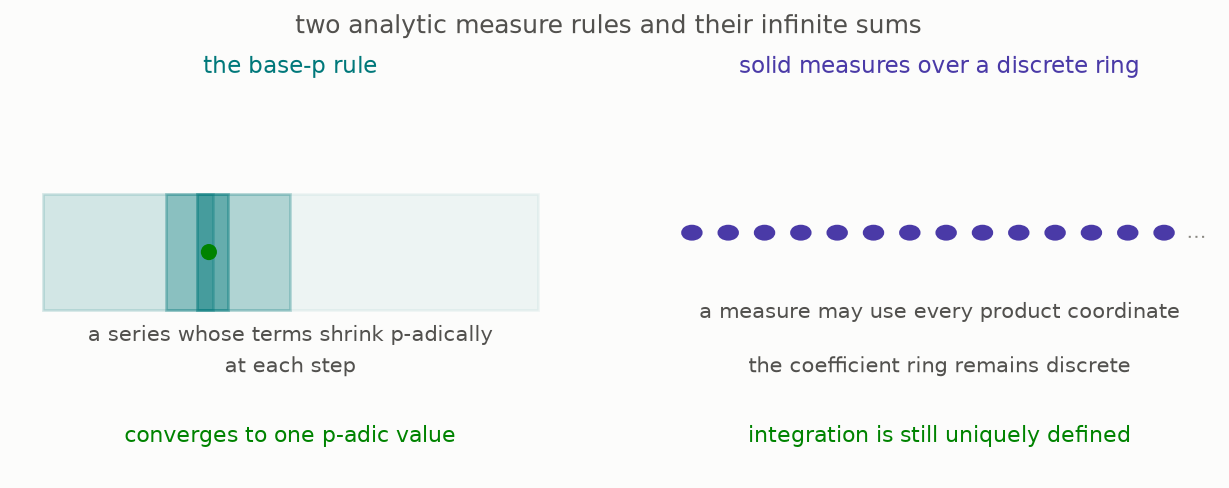
The p-adic measure rule and the solid rule over a discrete ring are shown with one example for each

A discrete ring has no nontrivial limits inside the ring itself, but the second example is still meaningful. The measure rule governs condensed modules over the ring, not only individual elements of the ring. Those modules can carry topological information in their probe values. The rule selects modules in which solid measures can be integrated consistently.

This separation is useful. The ring controls multiplication, while its measure theory controls infinite additive behavior in modules. We can change the completion rule without changing the algebraic formulas for multiplication.

A wider construction starts with a ring $A$ and a subring $A^+$ whose elements are declared to have size at most one (Remark 7.9, page 49). The pair $(A,A^+)$ is called a Huber pair. For the field of $p$-adic numbers, it gives bounded $p$-adic-valued measures. We will return to Huber pairs when we build geometric patches in chapter 6.

The mathematics

Proposition 7.8, page 48 of the lectures says that the following two measure theories are analytic:

$$ \mathbb Z_{p,\blacksquare}[S] :=\varprojlim_i\mathbb Z_p[S_i] =M(S,\mathbb Z_p), $$

$$ (A,\mathbb Z)^{\blacksquare}[S] :=\mathbb Z[S]^{\blacksquare}\otimes_{\mathbb Z}A \qquad\text{for a discrete ring }A. $$

Remark 7.9, page 49 extends the pattern to a Huber pair $(A,A^+)$ and gives

$$ (\mathbb Q_p,\mathbb Z_p)^{\blacksquare}[S] =M_b(S,\mathbb Q_p) =M(S,\mathbb Z_p)[1/p]. $$

Reading the symbols. The probe $S$ has finite stages $S_i$. The inverse limit $\varprojlim$ keeps compatible $p$-adic weights at every stage. The group $\mathbb Z_p$ is the $p$-adic integers, and $M(S,\mathbb Z_p)$ is the module of $\mathbb Z_p$-valued measures. In the second display, $A$ is a discrete ring. The tensor product $\otimes_{\mathbb Z}$ changes integer coefficients to coefficients in $A$. The black square marks the solid measure rule. A Huber pair consists of a ring $A$ and a chosen bounded subring $A^+$. The field $\mathbb Q_p$ is the $p$-adic numbers. The subscript $b$ means bounded, and $[1/p]$ permits division by powers of $p$.

Why it matters. These examples keep multiplication and summation separate. One framework handles a topological $p$-adic ring and a discrete ring without pretending that they have the same completion.

In the simulation. The selector switches between the two constructions. Nested boxes represent compatible $\mathbb Z_p$-valued weights. A row of coefficients represents the extension of $\mathbb Z[S]^{\blacksquare}$ from integer coefficients to a discrete ring $A$.

Use the controls to change the picture. Open the activity on its own page

3 · A measure rule for the real numbers

The integer-based solidification from part two sends the usual real line to zero. Real analysis therefore needs a different theory of measures. A natural place to begin is with finite lists of signed real weights and a rule that bounds their size.

Choose a positive exponent $p$. At $p=1$, add the absolute values of the weights. At $p=2$, square the absolute values, add them, and take a square root. Other positive exponents use the same pattern. This is the familiar $\ell^p$ size of a finite list.

A measure on a probe must agree across stages. Passing from a fine stage to a coarse one merges boxes and adds their weights. If a fine list is within a chosen size limit, the merged list must stay within the same limit. Otherwise, the allowed regions at different stages do not form an inverse system.

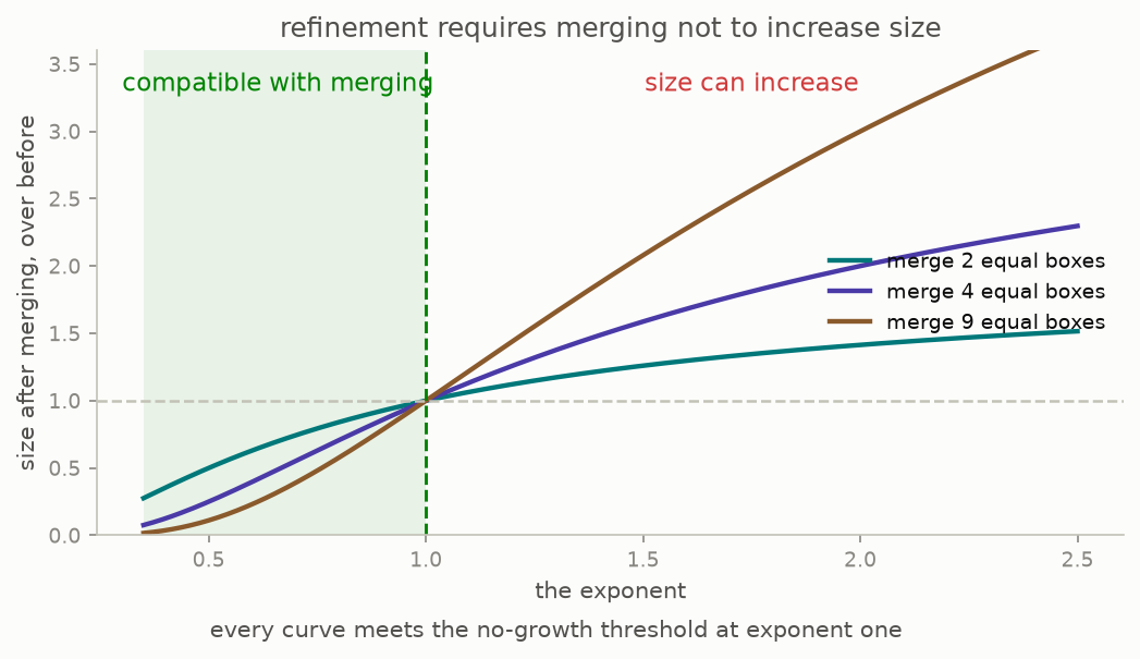
Curves for merging two, four, and nine equal boxes meet the no-growth level at exponent one

For equal weights, the effect can be calculated exactly. Merging does not increase size precisely when $p\le1$. Above one, the growth becomes larger as more boxes are merged. For example, joining four equal weights at $p=2$ doubles the size (Example 7.10, page 49).

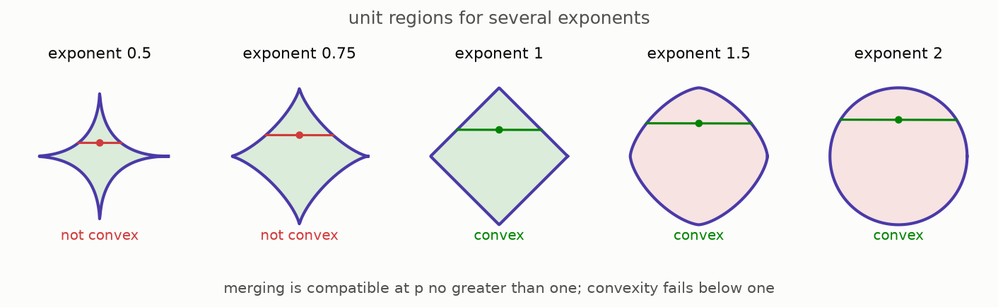
Five unit regions are convex at exponents at least one and bend inward below one

The same boundary causes a second difficulty. At and above one, the unit region is convex. Below one, it bends inward and is not convex. Classical functional analysis is largely based on locally convex spaces, but compatibility under merging forces us to use exponents at most one.

The fixed rule at $p=1$ gives the usual bounded signed measures, but it is not an analytic ring. Ribe found an extension of complete locally convex spaces whose middle term is not locally convex, so these spaces are not stable under the extensions required by the analytic condition (Example 7.10, page 49). Choosing one fixed exponent below one does not remove the related obstruction.

The successful construction does not fix a single smaller exponent. For a target $p\le1$, it combines the measure modules for every exponent $q<p$ into a directed union, or colimit. Theorem 7.11, page 50 proves that this varying-exponent construction is analytic. Its complete modules are called liquid modules.

The restriction $p\le1$ came from a finite operation: merging child boxes adds their weights. This is a recurring feature of condensed mathematics. Compatibility between finite stages places a strong condition on the infinite analytic theory.

The mathematics

Choose $0<p\le1$. Example 7.10, page 49 of the lectures defines the finite-stage size and measure module by

$$ \|(x_i)\|_{\ell^p}=\left(\sum_i|x_i|^p\right)^{1/p}, \qquad \mathcal M_p[S]=\bigcup_{r>0}\varprojlim_i \{x\in\mathbb R[S_i]\mid\|x\|_{\ell^p}\le r\}. $$

Equal weights make the effect of merging easy to calculate. For $n$ equal positive weights, the size changes by

$$ \frac{\|\text{after}\|_{\ell^p}}{\|\text{before}\|_{\ell^p}} =n^{1-1/p}\le1\quad\Longleftrightarrow\quad p\le1. $$

No fixed $p$ gives an analytic ring. Theorem 7.11, page 50 instead uses all smaller exponents:

$$ \mathcal M_{<p}[S]:=\varinjlim_{q<p}\mathcal M_q[S], \qquad (\mathbb R,\mathcal M_{<p})\text{ is an analytic ring.} $$

Reading the symbols. The exponent $p$ is positive and at most one. The list $(x_i)$ contains the weights on one finite stage. The absolute-value bars measure each real weight. The summation sign adds their $p$th powers, and the outside exponent $1/p$ defines the $\ell^p$ size. The union over $r>0$ allows any finite bound. The inverse limit $\varprojlim$ requires compatibility among the stages $S_i$. The fraction compares the size after merging with the size before merging. The double arrow $\Longleftrightarrow$ means “if and only if.” The direct limit $\varinjlim_{q<p}$ combines all positive exponents $q$ below $p$. The pair $(\mathbb R,\mathcal M_{<p})$ is the real ring with this combined measure rule.

Why it matters. Compatibility under refinement forces $p\le1$, exactly where local convexity is no longer available below the endpoint. Combining all smaller exponents gives the liquid theory that passes the analytic-ring test.

In the simulation. One control changes $p$, and another changes the number $n$ of merged boxes. The chart calculates $n^{1-1/p}$. A second picture shows whether the unit region is convex. These are separate conditions that meet at $p=1$.

Use the controls to change the picture. Open the activity on its own page

4 · Global functions and boundary tails

We now move from analysis to geometry. Begin with the affine line, whose global functions are polynomials in one coordinate $T$. To describe behavior near infinity, use the reciprocal coordinate $T^{-1}$. When $T$ becomes large, $T^{-1}$ becomes small, so series in $T^{-1}$ describe a formal neighborhood of the boundary.

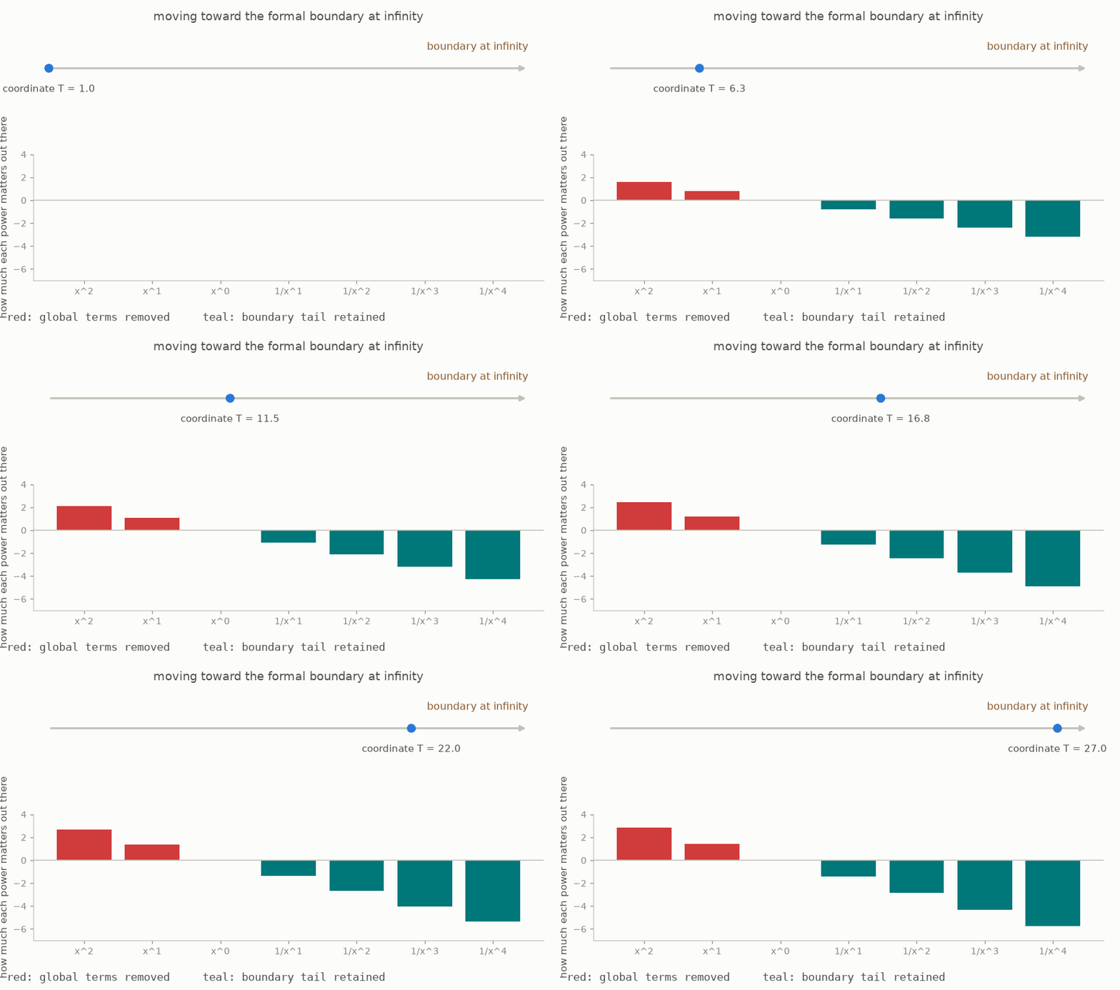
As a point moves toward infinity, bars compare powers of the coordinate with powers of its reciprocal

A formal Laurent series near infinity can have finitely many positive powers of $T$ and infinitely many negative powers. We will call this the boundary ring. Every polynomial has an expansion in this ring, but the boundary ring also contains infinite negative-power tails that no polynomial can contain.

Taking the quotient of the boundary ring by the polynomial ring removes all functions already defined globally. What remains records information that exists only near the boundary. This quotient becomes the basic ingredient for compactly supported cohomology in the next chapter.

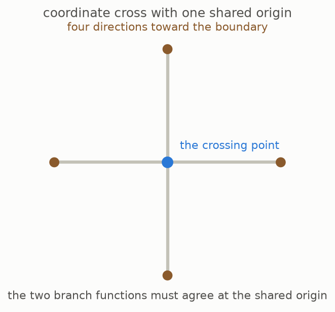
Two coordinate axes meet at one point and create four directions toward the boundary

The lectures also calculate the coordinate cross, which consists of two axes meeting at the origin (Remark 8.5, page 54). Each axis contributes its own Laurent tail. The two global polynomial descriptions must agree at the shared point. In the finite truncation used here, the quotient contains the tails from both branches plus one extra contribution from that shared relation. The count remains stable when the truncation is extended.

The mathematics

The affine line has global polynomial functions and formal functions near infinity. With coordinate $T$, Lecture VIII writes these rings as

$$ A=\mathbb Z[T], \qquad A_\infty=\mathbb Z((T^{-1})), \qquad A_\infty/A=\mathbb Z((T^{-1}))/\mathbb Z[T]. $$

The coordinate cross needs one copy of the boundary ring for each branch. Remark 8.5, page 54 of the lectures gives

$$ A=\mathbb Z[X,Y]/(XY), \qquad A_\infty=\mathbb Z((X^{-1}))\times\mathbb Z((Y^{-1})), $$

$$ A_\infty/A= \frac{\mathbb Z((X^{-1}))\times\mathbb Z((Y^{-1}))} {\mathbb Z[X,Y]/(XY)}. $$

Reading the symbols. The ring $A=\mathbb Z[T]$ contains polynomials in $T$ with integer coefficients. The double parentheses in $\mathbb Z((T^{-1}))$ mean formal Laurent series in the inverse coordinate. These series may have infinitely many negative powers of $T$ but only finitely many positive powers. The subscript $\infty$ marks functions near the boundary. The quotient $A_\infty/A$ identifies two boundary series when they differ by a global polynomial. For the cross, $X$ and $Y$ are its two coordinates. The relation $XY=0$ restricts points to one axis or the other. The product $\times$ keeps one Laurent series for each branch.

Why it matters. The quotient removes every function that already extends over the whole affine space. It keeps only boundary information. On the cross, the relation at the shared origin links the two branches and creates the additional contribution seen in the finite model.

In the simulation. Moving toward the boundary increases $T$ and decreases $T^{-1}$. Polynomial terms belong to $A$ and disappear in the quotient. Negative-power tails remain in $A_\infty/A$.

Use the controls to change the picture. Open the activity on its own page

5 · Compactly supported cohomology

A map from a space to a point gives two ways to collect information. Ordinary pushforward collects global sections across the whole space. Pushforward with compact support keeps the part whose support does not continue out toward the boundary.

For the second operation, we must compare functions defined everywhere with functions that exist near the boundary. The quotient from chapter 4 provides exactly this comparison.

Global function blocks are removed from boundary function blocks, leaving the negative-power tails

For a finitely generated algebra over the integers, the global module theory and the boundary module theory are connected by three adjoint functors. The new left adjoint is built from the boundary quotient. This construction works because the relevant measure theories are analytic, so limits, products, and derived operations stay in the appropriate complete categories (Theorem 8.1, page 53).

The resulting compactly supported pushforward has a right adjoint (Theorem 8.2, page 53). In standard notation, they are lower shriek $f_!$ and upper shriek $f^!$. Applying $f^!$ to the unit object gives the dualizing complex. This adjunction defines the object by a universal property instead of requiring a separate guess in every example.

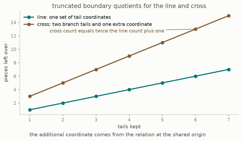
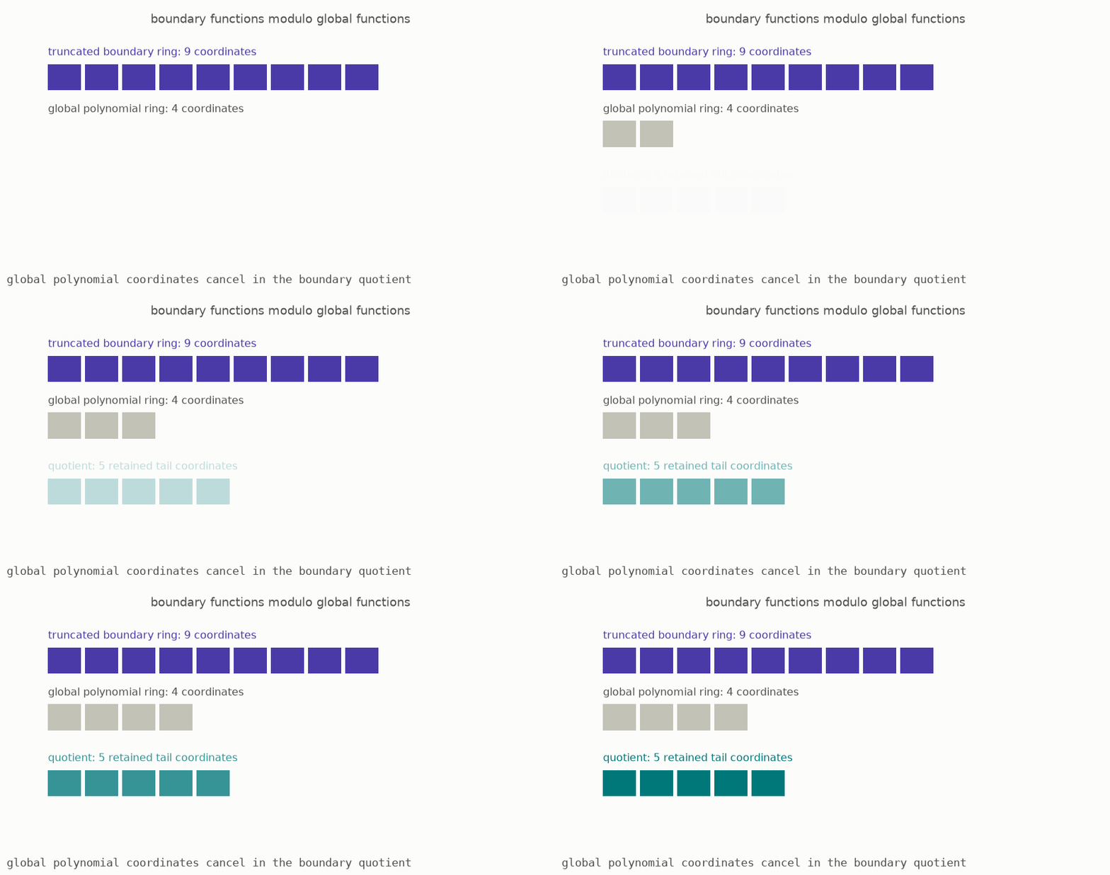
A chart compares finite truncations of the boundary quotient for a line and a coordinate cross

For the coordinate cross, the lectures describe the dualizing complex as the integer dual of the quotient of boundary functions by global functions (Remark 8.5, page 54). The code only reproduces the rank pattern in finite truncations. It does not verify the categorical theorem.

Condensed modules are needed because boundary tails involve infinite products. Compactly supported pushforward can therefore send a discrete module to a genuinely nondiscrete object (the discussion after Theorem 8.2, page 53). Its right adjoint does preserve discrete objects, so the final dualizing complex can still be classical even though its construction passes through a larger category.

Compactly supported pushforward also preserves compact objects. After gluing the local construction, proper pushforward agrees with compactly supported pushforward. This turns formal compactness into the usual finiteness result for coherent cohomology (Remark 8.3, page 54).

The mathematics

Let $A$ be a finitely generated integer algebra. Theorem 8.1, page 53 of the lectures constructs

$$ j_!\dashv j^*\dashv j_*: D(A^{\blacksquare})\longleftrightarrow D((A,\mathbb Z)^{\blacksquare}). $$

Let $f:\operatorname{Spec}A\to\operatorname{Spec}\mathbb Z$ be the projection. Theorem 8.2, page 53 defines compactly supported pushforward and its right adjoint:

$$ f_!:D(A^{\blacksquare})\longrightarrow D(\mathbb Z^{\blacksquare}), \qquad f_!\dashv f^!, $$

The same theorem identifies the dualizing complex:

$$ \omega_A:=f^!\mathbb Z \cong R\!\operatorname{Hom}_{\mathbb Z}(f_!A,\mathbb Z). $$

Reading the symbols. The ring $A$ is finitely generated over the integers. The notation $D$ means a derived category of modules with the measure rule shown in parentheses. The symbols $j_!$, $j^$, and $j_$ are functors. The symbol $\dashv$ means “is left adjoint to.” The map $f$ sends the affine space $\operatorname{Spec}A$ to the base $\operatorname{Spec}\mathbb Z$. The functor $f_!$ is pushforward with compact support, and $f^!$ is its right adjoint. The object $\omega_A$ is the dualizing complex. The expression $R\!\operatorname{Hom}_{\mathbb Z}$ is the derived integer dual. The symbol $\cong$ means a canonical isomorphism.

Why it matters. The boundary quotient provides the new left adjoint $j_!$. It is used to construct $f_!$, and the right adjoint $f^!$ then defines the dualizing complex. The theorem also says that $f_!$ preserves compact objects, although it generally does not preserve discrete objects.

In the simulation. Choose the line or the cross. The top row represents boundary functions, the middle row represents global functions, and the bottom row represents their quotient. The displayed number is a finite truncation of the construction, not a proof of the adjunction.

Use the controls to change the picture. Open the activity on its own page

6 · Gluing affine patches

So far, we have worked with one ring, which describes one affine patch. A general geometric space is built from several patches that overlap. To glue the module theories, each patch must remember both its ring of functions and which functions count as bounded.

A Huber pair consists of a ring $A$ and an integrally closed subring $A^+$. Elements of $A^+$ are declared to have size at most one. A point of the corresponding valuation space assigns multiplicative sizes to all elements of $A$ while keeping every element of $A^+$ within that bound (Proposition 9.2, page 63).

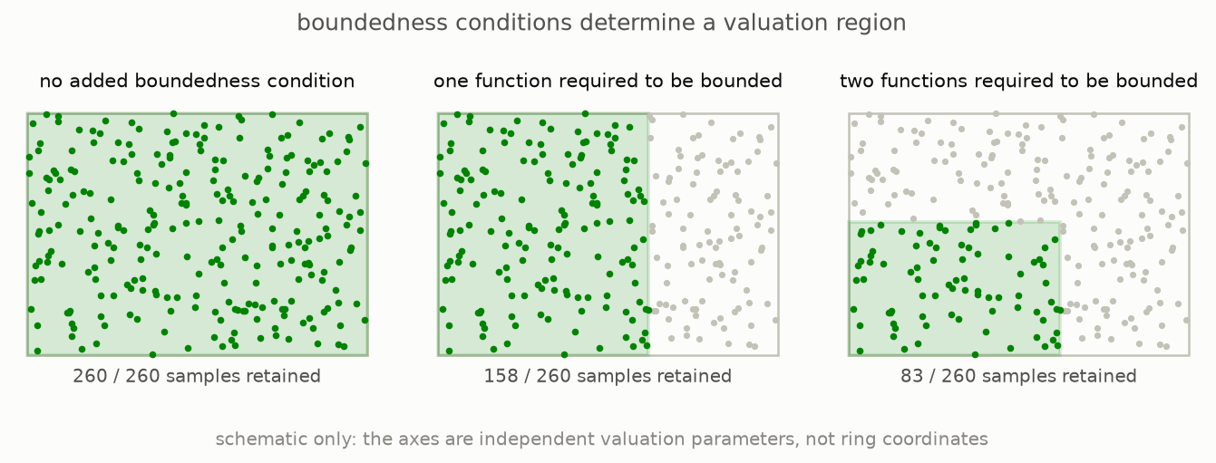
Three regions of possible valuations become smaller as more functions are required to have size at most one

Choosing $A^+$ selects the valuations that regard all its elements as bounded. In the setting of the proposition, the selected region also recovers $A^+$: it consists exactly of the functions whose size is at most one at every point in the region. The algebraic choice and the geometric region determine each other.

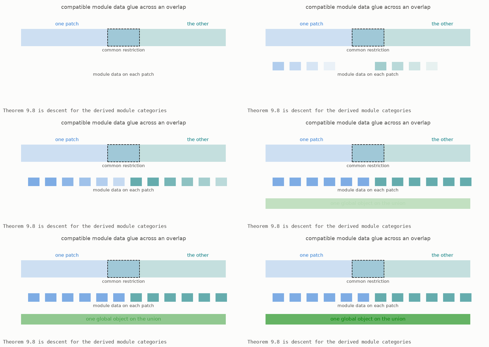
Compatible module data on two overlapping affine patches combine into one object on their union

Theorem 9.8, page 65 says that the derived categories of complete modules form a sheaf over these patches. Local module objects that agree on every overlap determine one global object, including all required higher compatibility data. This theorem lets us extend the affine construction of compactly supported cohomology to spaces made from many affine pieces.

The statement uses infinity-categories because gluing derived objects needs more than maps up to homotopy. It must also retain compatible homotopies between homotopies and all further levels. Earlier finite examples did not need this language, but the global gluing step does.

The proof follows the usual pattern of Zariski descent. Cover a space by patches where selected functions become invertible, verify the statement on each localized patch, and show that an object vanishing on every patch was already zero globally. Lecture X proves the localization facts needed for this argument.

The mathematics

For a ring $A$, Proposition 9.2, page 63 of the lectures relates an integrally closed subring $A^+$ to its valuation region:

$$ \operatorname{Spa}(A,A^+) =\{x\in\operatorname{Spv}(A)\mid |f(x)|\le1\text{ for every }f\in A^+\}, $$

$$ A^+=\{f\in A\mid |f(x)|\le1\text{ for every }x\in\operatorname{Spa}(A,A^+)\}. $$

Theorem 9.8, page 65 states the gluing result:

$$ U=\operatorname{Spa}(A,A^+) \longmapsto D((A,A^+)^{\blacksquare}) \quad\text{is a sheaf of }\infty\text{-categories on }X. $$

Reading the symbols. The subring $A^+$ contains the functions declared to have size at most one. The space $\operatorname{Spv}(A)$ contains equivalence classes of valuations on $A$. The region $\operatorname{Spa}(A,A^+)$ keeps the valuations that bound every element of $A^+$ by one. The braces mean “the set of,” $\in$ means “belongs to,” and the vertical bar means “such that.” The expression $|f(x)|$ is the size that the valuation $x$ assigns to $f$. The open patch is $U$, and $D((A,A^+)^{\blacksquare})$ is its derived category of complete modules. Saying that these categories form a sheaf means that compatible local objects glue uniquely. The infinity symbol records all higher homotopies needed for that compatibility.

Why it matters. The first two displays say that the bounded subring and its valuation region determine one another. The theorem then lets the module categories on local regions assemble into one global category.

In the simulation. Selecting bounded functions changes $A^+$. Highlighted points are the valuations that satisfy the corresponding bounds. The plotted points are a schematic model, so they show how extra conditions shrink a region rather than representing the valuation space of one specific ring.

Use the controls to change the picture. Open the activity on its own page

7 · The six operations

The local and global constructions fit into the six-operations formalism, a standard framework for cohomology theories. Each space receives a category of sheaf-like objects. A map of spaces then gives operations that combine these objects or move them between the source and target.

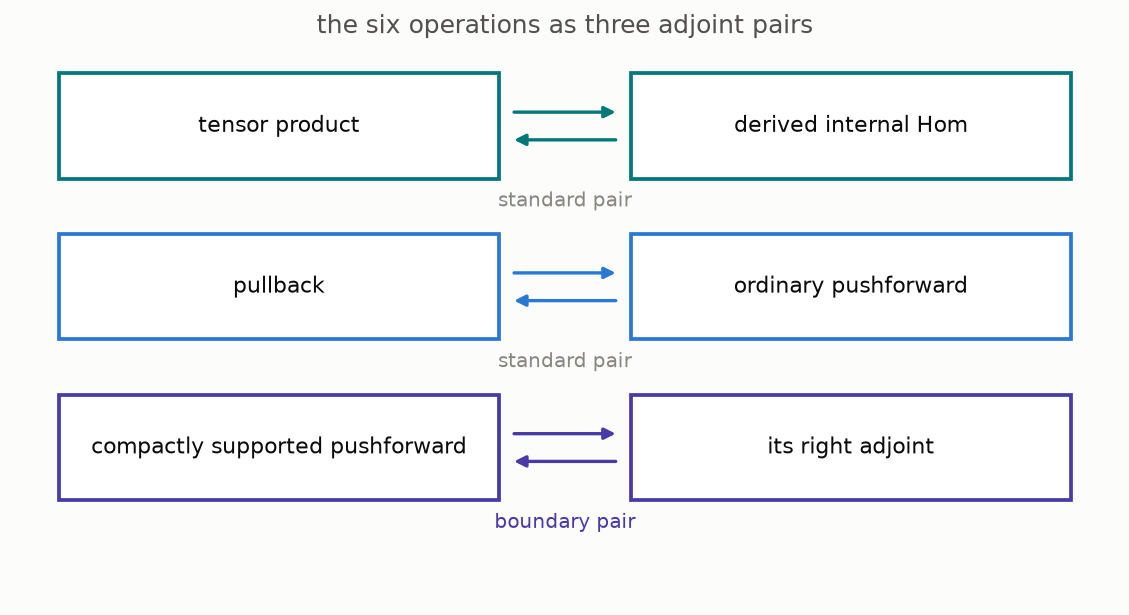
Tensor with internal Hom, pullback with pushforward, and lower shriek with upper shriek form three adjoint pairs

The six operations form three pairs. In each pair, the left operation is adjoint to the right one. This means that maps formed after applying one operation correspond naturally to maps formed with its partner.

Tensor product and internal Hom. Tensor product combines two objects on the same space. Internal Hom records maps from one object into another.

Pullback and ordinary pushforward. For a map of spaces, pullback moves an object from the target to the source. Ordinary pushforward moves information from the source back to the target and is the right adjoint of pullback.

Compactly supported pushforward and upper shriek. Lower shriek pushes information forward while controlling what happens at the boundary. Upper shriek is its right adjoint. Applied to the unit, upper shriek gives the dualizing object.

The first four operations already exist in ordinary derived algebraic geometry. The difficult construction is compactly supported pushforward, which uses the boundary theory from chapter 5. Once $f_!$ exists, its right adjoint $f^!$ completes the third pair (the discussion after Theorem 11.1, page 72).

Two special cases guide the definition. If a map is proper, no support can escape through a boundary, so compactly supported pushforward equals ordinary pushforward. For an open inclusion, lower shriek is extension by zero. Nagata compactification expresses a separated finite-type map as an open inclusion followed by a proper map. These rules determine a candidate for $f_!$, while the theorem must still prove that it does not depend on the chosen factorization and that it behaves coherently under composition.

The mathematics

The discussion after Theorem 11.1, page 72 of the lectures arranges the operations into three adjoint pairs:

$$ -\otimes_X B\dashv R\!\operatorname{Hom}_X(B,-), \qquad f^*\dashv f_*, \qquad f_!\dashv f^!. $$

Two required identities are

$$ f_!\cong f_*\quad\text{when }f\text{ is proper}, \qquad f^!\cong f^*\quad\text{when }f\text{ is étale}. $$

The projection formula is

$$ f_!(A\otimes_X f^*B)\cong f_!A\otimes_Y B. $$

Reading the symbols. The tensor product $\otimes_X$ combines objects on $X$. The derived internal Hom $R\!\operatorname{Hom}_X$ records maps from $B$. The map of spaces is $f:X\to Y$. Its pullback is $f^$, ordinary pushforward is $f_$, compactly supported pushforward is $f_!$, and the right adjoint of $f_!$ is $f^!$. The symbol $\dashv$ means that the left operation is left adjoint to the right one. The symbol $\cong$ means naturally isomorphic. Proper maps have no escaping boundary contribution. Étale maps satisfy the local condition under which upper shriek agrees with pullback. In the projection formula, $A$ is an object on $X$ and $B$ is an object on $Y$.

Why it matters. The first four operations are already available in ordinary derived geometry. The boundary construction supplies $f_!$, and its adjoint supplies $f^!$. The listed identities make this new pair compatible with the existing operations.

In the simulation. Choose one of the six operations to see its source, target, and adjoint partner. Proper and nonproper examples show when $f_!$ agrees with $f_*$ and when boundary contributions must be removed.

Use the controls to change the picture. Open the activity on its own page

8 · Coherent duality

Duality pairs two kinds of cohomological information and produces a scalar on the base. A perfect pairing loses no information: knowing how one input pairs with every input on the other side determines it completely. For a smooth space, the partner uses differential forms and a shift by the dimension.

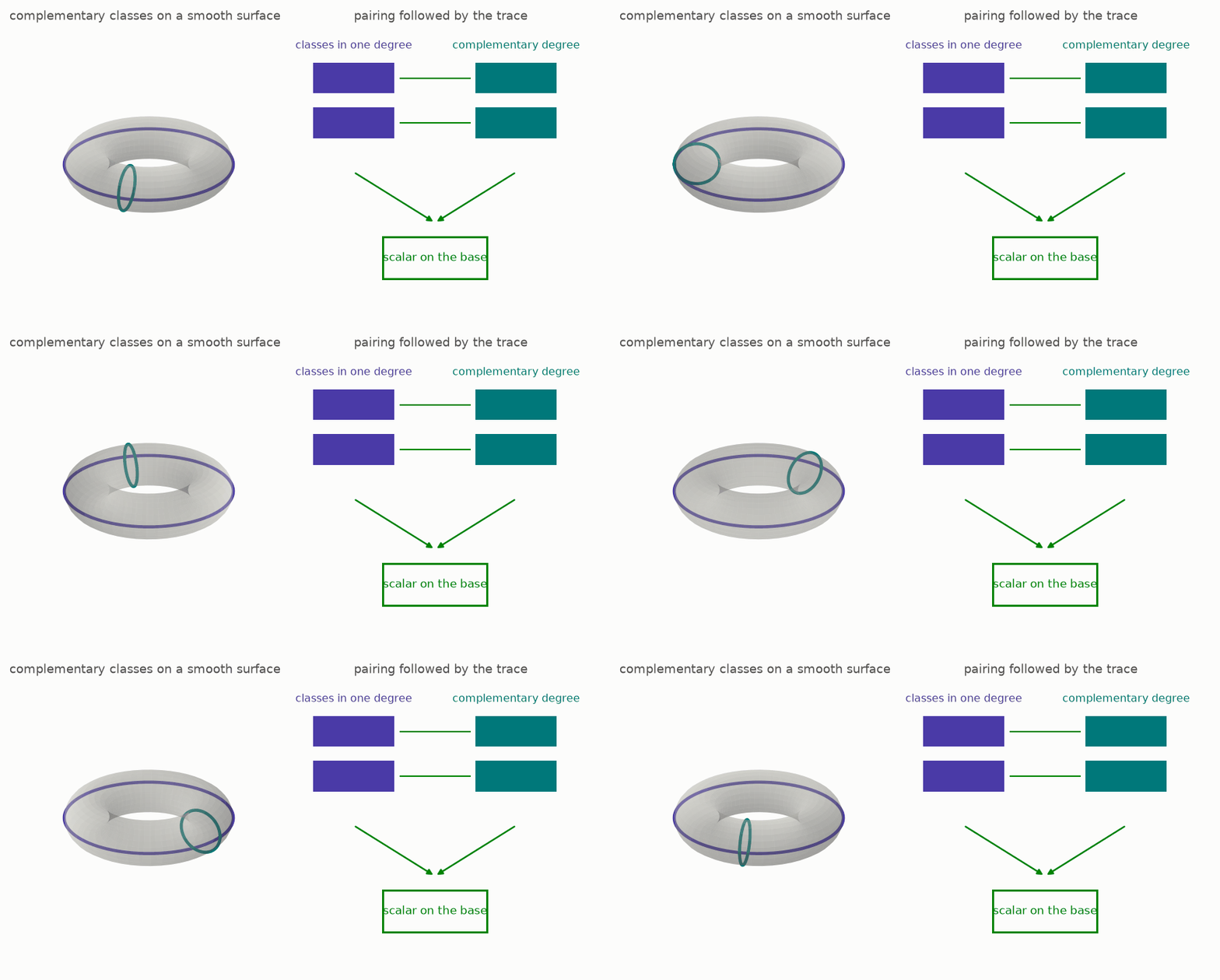
A torus rotates while classes in complementary degrees pair and pass through a trace map

The animation models this on a surface. One class has a chosen degree, and its partner has the complementary degree. Their product reaches the top degree. Compactly supported pushforward carries that class to the base, where a trace map turns it into one scalar.

Theorem 11.1, page 71 applies to a separated smooth map of finite type with a fixed relative dimension. It constructs compactly supported pushforward, proves that it agrees with ordinary cohomology for a proper map, and gives a canonical trace from top-degree differential forms to the base. Pairing with that trace identifies the two dual objects. This is coherent duality in the setting of solid modules.

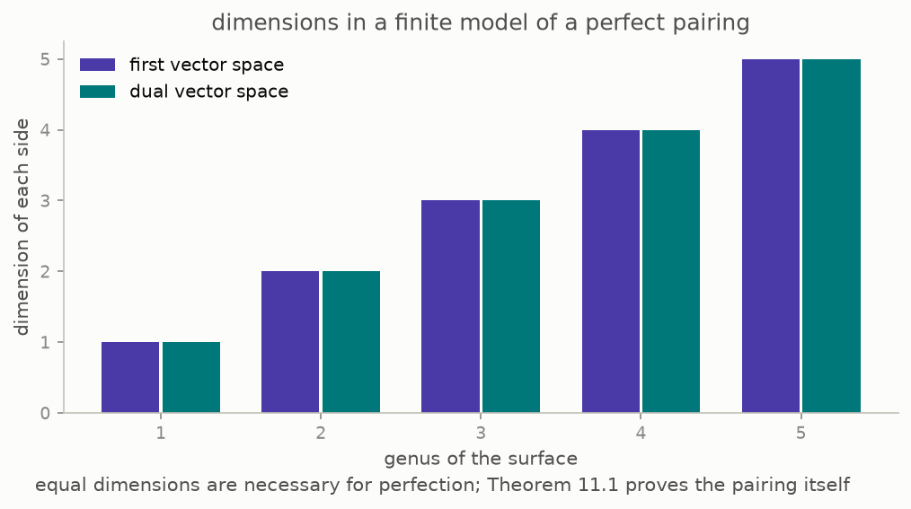
Matching spaces of degree-zero and degree-one classes pair into a top-degree class and then into the base ring

The earlier chapters provide three parts of the construction. First, $f^!$ is defined as the right adjoint of compactly supported pushforward, so $f^!$ of the unit is the dualizing complex. In the smooth case, the theorem identifies this object with the expected differential forms and proves that the pairing is perfect.

Second, compactly supported pushforward preserves compact objects. For a proper map, it agrees with ordinary pushforward, which also preserves discreteness. This recovers the classical finite-generation statement for coherent cohomology (Remark 8.3, page 54).

Third, the construction may pass through nondiscrete modules because boundary functions have infinite tails. The right adjoint can return the dualizing complex to the discrete setting. Condensed mathematics provides the larger category needed for the middle of the construction.

The mathematics

Theorem 11.1, page 71 of the lectures considers a separated smooth map $f:X\to\operatorname{Spec}R$ of finite type and relative dimension $d$. Define

$$ \omega_{X/R}:=\bigwedge^d\Omega^1_{X/R}, $$

The theorem gives a trace and a perfect duality:

$$ \operatorname{tr}:f_!\omega_{X/R}[d]\longrightarrow R, $$

$$ R\!\operatorname{Hom}_{X}(C,\omega_{X/R})[d] \xrightarrow{\sim} R\!\operatorname{Hom}_{R}(f_!C,R). $$

Properness removes the difference between compactly supported and ordinary cohomology. When $f$ is proper, the theorem also gives

$$ f_!C\cong R\Gamma(X,C). $$

Reading the symbols. The space is $X$, the base ring is $R$, and $\operatorname{Spec}R$ is its affine base space. The integer $d$ is the relative dimension. The module $\Omega^1_{X/R}$ contains relative differential one-forms. Its top exterior power $\bigwedge^d$ is written $\omega_{X/R}$. The functor $f_!$ is compactly supported pushforward. Square brackets $[d]$ shift the cohomological degree by $d$. The trace $\operatorname{tr}$ sends a top-degree compactly supported class to a scalar in $R$. The letter $C$ names a suitable complex on $X$. The two derived Hom expressions are dual objects, and the arrow marked $\sim$ says that the trace pairing identifies them. The notation $R\Gamma(X,C)$ means derived global cohomology.

Why it matters. The theorem identifies the right adjoint of compactly supported cohomology with the expected object of differential forms and proves that the pairing loses no information. If the space is proper, compactly supported and ordinary cohomology agree, which recovers classical coherent duality.

In the simulation. Degree controls choose a class and a possible partner. Their product reaches the top degree only when the degrees add to the displayed dimension $d$. The trace then sends the result to one scalar. Matching finite dimensions illustrate a perfect pairing but do not prove the theorem.

Use the controls to change the picture. Open the activity on its own page

What the three parts established

The guide followed one continuous path. Probes first moved topological information into algebra by recording continuous families of points. Compatible integer measures then gave solid groups a precise rule for infinite sums. Finally, analytic rings allowed each ring to carry a suitable theory of measures. This made it possible to build local geometry, glue it globally, define compactly supported cohomology, and obtain coherent duality from an adjunction.

The lectures record a course taught in 2019 and were published in this form in May 2026. Their preface points to later work by Clausen and Scholze on broader analytic rings, real and complex variants, light condensed mathematics, and analytic stacks. They also include an appendix proving the universal resolution used in Lecture IV (Remark 4.6, page 25). This guide introduces the progression of ideas, but the lectures contain the full statements and proofs.

How this part lines up with the lectures

this guide	in the lectures
chapter 1, rings and measure rules	Definition 7.1, page 45; Definition 7.4, page 46
chapter 2, two analytic examples	Proposition 7.8, page 48; Remark 7.9, page 49
chapter 3, the real measure rule	Example 7.10, page 49; Theorem 7.11, page 50
chapter 4, boundary functions	Lecture VIII from page 53; Remark 8.5, page 54
chapter 5, compact support	Theorem 8.1 and Theorem 8.2, page 53; Remarks 8.3 to 8.5, page 54
chapter 6, gluing	Proposition 9.2, page 63; Theorem 9.8, page 65; Lecture X from page 66
chapter 7, the six operations	the discussion after Theorem 11.1, page 72
chapter 8, coherent duality	Theorem 11.1, page 71; Remark 8.4, page 54

Checking it yourself

The following commands rerun the finite calculations and rebuild their figures. They do not prove the categorical theorems quoted from the lectures.

cd condensed-math
make venv
make test
make figures

For this part, the tests:

calculate how merging equal weights changes their $\ell^p$ size and locate the boundary at $p=1$
verify the formula that the merge ratio is the number of boxes raised to one minus the reciprocal of $p$
check that the unit region is convex at and above one and not convex below one
count truncated boundary tails for the line and coordinate cross
confirm that the cross keeps one extra contribution beyond the tails from its two branches
verify that these rank counts remain stable when the truncation is extended

The analytic-ring theorem, gluing theorem, six-operations formalism, and duality theorem concern entire categories. They are quoted from the lectures and cannot be established by these finite tests. The file notes/research-content.md separates those quotations from the calculations used in the activities.

Glossary

phrase used in this guide	standard mathematical term
a ring with a compatible measure rule	an analytic ring
the legal measures on each probe	a theory of measures
a unit weight at one point	a Dirac measure
the exponent in the size formula	the $p$ in an $\ell^p$ norm or quasinorm
combining all smaller exponents	the colimit that defines the liquid theory
functions near infinity	formal Laurent series in the inverse coordinate
a negative-power tail	the boundary part of a Laurent expansion
collection with support away from the boundary	cohomology with compact support
compactly supported pushforward	lower shriek, $f_!$
the right adjoint of compactly supported pushforward	upper shriek, $f^!$
the object obtained by applying $f^!$ to the unit	the dualizing complex
a ring with a chosen bounded subring	a Huber pair $(A,A^+)$
the region defined by multiplicative sizes	a valuation space
local objects that agree and combine globally	descent for a sheaf of categories
tensor, internal Hom, pullback, pushforward, and the shriek pair	the six operations
the final map from top-degree data to the base	the trace map
no contribution can escape through the boundary	properness

1 · A ring and its legal measures

The mathematics

2 · Two analytic examples

The mathematics

3 · A measure rule for the real numbers

The mathematics

4 · Global functions and boundary tails

The mathematics

5 · Compactly supported cohomology

The mathematics

6 · Gluing affine patches

The mathematics

7 · The six operations

The mathematics

8 · Coherent duality

The mathematics

What the three parts established

How this part lines up with the lectures

Checking it yourself

Glossary

Further reading