Condensed mathematics, part 1 of 3
Understanding Spaces Through Probes
This is the first of three parts on condensed mathematics. We begin with a simple problem: the same set of numbers can have different rules for which numbers are close. Ordinary algebra does not handle that difference well. We will build a new description of a space, one step at a time, and use it to repair the problem. You do not need any previous mathematics.
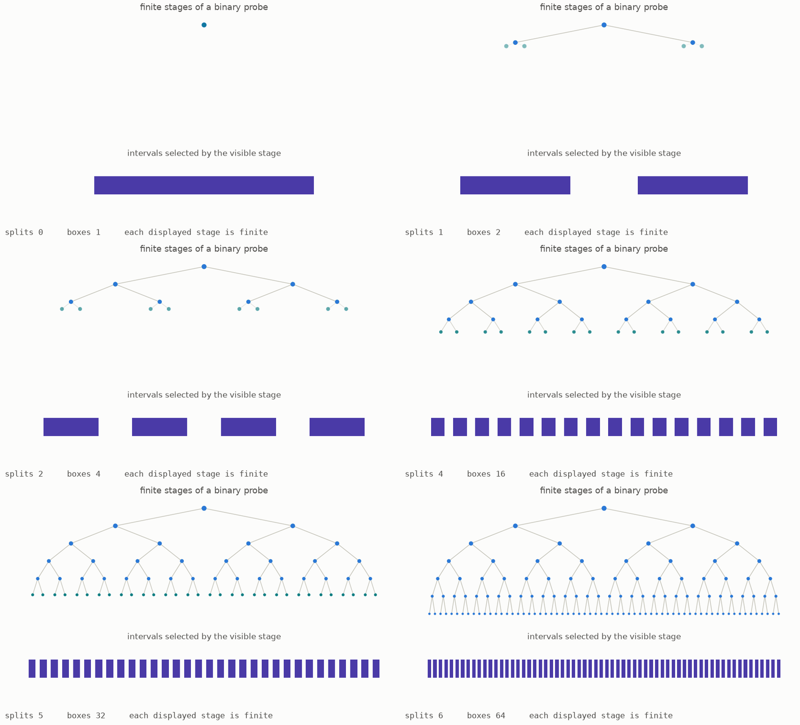
The animation shows the basic object used in this guide. Start with one box. Divide it into smaller boxes, then divide those boxes again. Each stage has only finitely many boxes, so we can view and study it completely. If the process continues without end, a path through all the stages picks out a point. The whole branching pattern also records how the points are separated from one another.
We will call this object a probe. Its standard name is a profinite set. Instead of describing a space only by listing its points, condensed mathematics records every continuous way that every probe can map into the space. This extra information remembers which families of points are close.
This part covers Lectures I to III of Peter Scholze's Lectures on Condensed Mathematics (arXiv:2605.03658, May 2026). The lectures describe joint work with Dustin Clausen from a course taught in Bonn in 2019. Part two introduces infinite sums, and part three adds rings and geometry. You can find the text, figures, and code in the open source repository. Each chapter also has an activity in which changing a control updates the picture. You can open the full list of part-one activities at any time.
    first see the problem       1  the same numbers with different notions of closeness
    build the new description  2  finite stages that form a probe
                               3  continuous maps from a probe into a space
                               4  the cut and glue rules
    use the description         5  a quotient that points cannot detect
                               6  probes on which every cover splits
    compare with topology       7  recovering familiar spaces
8 keeping track of holes1 · The same numbers, but different ideas of closeness
Take two copies of the real numbers. The copies contain exactly the same values, but we give them different rules for closeness.
In the first copy, different numbers are never close. Every number stands alone. This is the real line with the discrete topology, which we will sometimes call the discrete real line. In the second copy, we keep the usual distance. Here 0.999 is close to 1, a sequence can approach a limit, and continuous motion is possible. This is the usual real line.
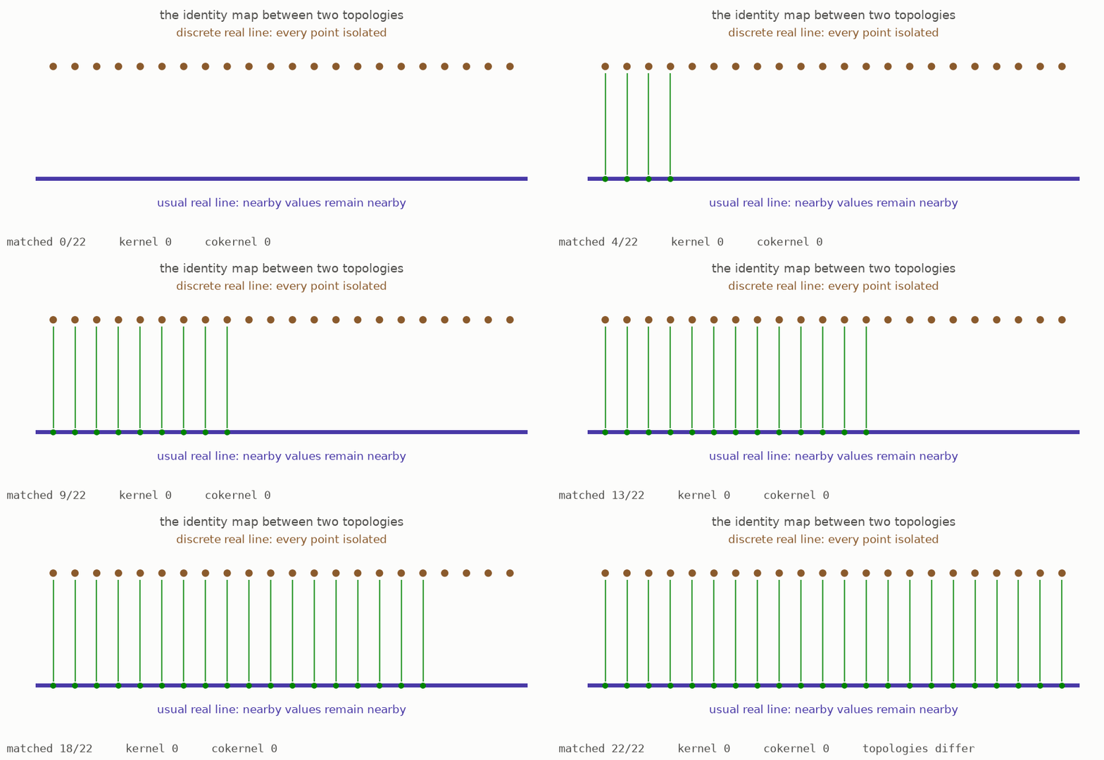
Map each number in the discrete copy to the same number in the usual copy. Every input has one output, no two inputs have the same output, and every output is reached. The map is therefore a bijection of sets.
The map is not an isomorphism of topological spaces. It is continuous from the discrete line to the usual line, but its inverse is not continuous. A single point is an open set in the discrete line. A single point is not open in the usual line. The inverse therefore fails the definition of continuity.
This creates a problem for algebra. For a map of abelian groups, the kernel consists of the elements sent to zero. The cokernel measures what remains in the target after we account for the image. In an abelian category, a map with zero kernel and zero cokernel must be an isomorphism. Our map has zero kernel and zero cokernel when treated as a map of topological abelian groups, but it is not an isomorphism. The usual category of topological abelian groups does not support this basic algebraic test.
The lectures begin with this failure (Example 1.9, page 9). Both real lines have the same individual points, so checking one point at a time cannot distinguish them. A useful replacement must also record how whole compact families of points move.
The mathematics
Example 1.9, page 9 of the lectures writes the identity map and its condensed cokernel explicitly. In topological abelian groups, the map has zero kernel and cokernel even though it is not an isomorphism:
After we pass to condensed abelian groups, the cokernel $Q$ is not zero. On a profinite probe $S$, it has the value
Reading the symbols. The symbol $\mathbb{R}$ means the real numbers. The subscript $\mathrm{disc}$ gives them the discrete topology. The label $\mathrm{id}$ means that every number maps to itself. The expressions $\ker$ and $\operatorname{coker}$ mean kernel and cokernel. The symbol $0$ is the zero group, and $\not\cong$ means “is not isomorphic to.” The letter $Q$ names the condensed cokernel. The symbol $*$ is the probe with one point. The notation $C(S,\mathbb{R})$ means all continuous maps from $S$ to the usual real line. The subscript $\mathrm{lc}$ keeps only the locally constant maps, which are exactly the continuous maps into the discrete real line. The fraction bar forms a quotient group. Finally, $\neq0$ says that this quotient contains a nonzero element for some probe.
Why it matters. A one-point probe sees $Q(*)=0$, while a larger probe can see $Q(S)\neq0$. The condensed cokernel keeps the topological information that pointwise algebra lost. Theorem 1.10, page 9 says that condensed abelian groups form an abelian category, so zero kernel and zero cokernel once again imply that a map is an isomorphism.
In the simulation. The upper row represents $\mathbb{R}_{\mathrm{disc}}$, and the lower row represents $\mathbb{R}$. Each vertical line connects one real value to itself under $\mathrm{id}$. The point-level kernel and cokernel remain zero even though the two rows use different rules for closeness.
2 · Building a probe from finite stages
We need probes that carry their own notion of closeness. To build one, start with a finite set of boxes and repeatedly divide each box into smaller boxes. At every stage, a map tells us which new box came from which box in the previous stage. The full probe consists of all the stages together with these maps.
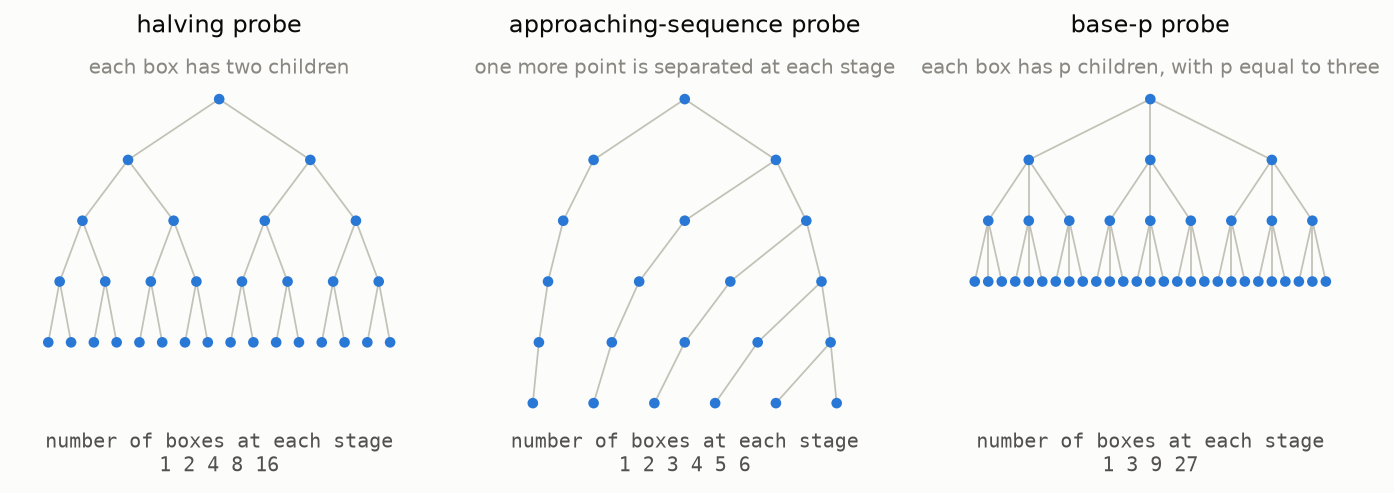
A point of the completed probe is a choice of one box at every stage, where each chosen box lies inside the one chosen before it. The lectures call this an inverse limit of finite sets, or a profinite set. We will use three examples throughout the guide.
The halving probe divides each box into two. After ten divisions, it has 1024 boxes. Its completed set of points is the Cantor set. The approaching-sequence probe contains a sequence and its limit. At stage five, the first five sequence points have separate boxes, while all later points and the limit remain together in one box. Each new stage separates one more point.
The base-$p$ probe divides each box into $p$ pieces. Its points form the $p$-adic integers. In that number system, divisibility by powers of $p$ determines which numbers are close. Part two uses this probe to show why one infinite sum can diverge under the usual distance and converge under the $p$-adic distance.
The code follows Definition 1.2, page 6 directly. It stores each finite set and each map to the earlier stage. The tests check the size of every stage and verify that moving back through several stages gives a consistent answer.
The mathematics
Definition 1.2, page 6 of the lectures defines a profinite set as an inverse limit of finite sets:
Reading the symbols. The letter $S$ names the complete probe, and $S_i$ is its finite stage numbered $i$. The symbol $\cong$ means “is isomorphic to.” The symbol $\varprojlim$ means inverse limit, so a point of $S$ is one compatible choice of a box at every stage. The map $\pi_{ji}$ sends a box at the finer stage $j$ back to its parent at stage $i$. The double-headed arrow says that every coarse box has a finer box above it. The inequalities put the stages in order. The symbol $\circ$ means composition. The last equality says that returning two stages at once gives the same result as returning one stage at a time.
Why it matters. The formula describes one infinite object using finite pieces and exact rules between them. The three examples differ only in their finite sets $S_i$ and their maps $\pi_{ji}$.
In the simulation. The depth control chooses the largest stage $i$ on the screen. Each row is a finite set $S_i$, and each branch shows part of the transition map $\pi_{i+1,i}$. Selecting one box highlights the finer boxes that map back to it.
3 · Mapping a probe into a space
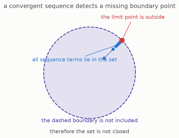
A probe lands in a space when we map all its points into the space continuously. Continuity requires the map to preserve closeness. For example, if points of the probe approach a limit, their images must approach the image of that limit.
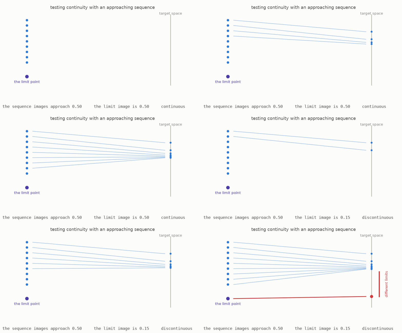
The animation compares two maps from the approaching-sequence probe. In the first map, the images of the sequence approach the chosen image of the limit, so the map is continuous. In the second map, the sequence approaches one value while the limit is sent to another. That map is not continuous.
We can now describe a space by recording every continuous map into it from every probe. For each probe, the record gives a set of allowed maps. This record is a condensed set once it satisfies the cut and glue rules in the next chapter (Definition 1.2, page 6). It remembers more than a list of points because it also tells us which compact families of points fit together continuously.
If the space supports addition, we can add two probe maps point by point and obtain a condensed group. If it also supports multiplication, we obtain a condensed ring (Example 1.3, page 7).
This description distinguishes the two real lines from chapter 1. The approaching probe has many continuous maps into the usual real line. A convergent sequence of real values and its limit give one. A map into the discrete real line can converge only if the sequence is eventually constant. The two lines therefore give different answers to the same probe.
For spaces whose topology comes from a distance, convergent sequences determine the topology. The approaching probe is enough to test those sequences (Remark 1.6, page 9). More general spaces need all profinite probes, but this example shows how a probe detects information that isolated points miss.
The mathematics
Example 1.3, page 7 of the lectures sends a topological space $X$ to the condensed set represented by it:
For the approaching probe $S=\mathbb{N}\cup\{\infty\}$, continuity has the following direct test:
Reading the symbols. The underline in $\underline{X}$ marks the condensed set associated with the space $X$. The expression $\underline{X}(S)$ is its answer to the probe $S$. The letter $C$ denotes continuous maps. The braces contain all maps $f$ from $S$ to $X$, and the vertical bar means “such that.” The symbol $\mathbb{N}$ means the natural numbers, and $\infty$ is the added limit point. The long arrow says that the images $f(n)$ approach $f(\infty)$ as $n$ grows without bound. Remark 1.6, page 9 explains why this test determines a metrizable space.
Why it matters. The one-point probe records only the points of $X$. Larger probes also record which families of points vary continuously. That is why they can distinguish the discrete and usual real lines.
In the simulation. One slider chooses the value approached by $f(n)$. The other chooses $f(\infty)$. The map passes the continuity test exactly when these values agree.
4 · The cut and glue rules
The answers for different probes must agree with one another. A condensed set follows two rules, called cut and glue. These are the two sheaf conditions in its definition.
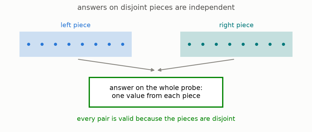
Cut. Suppose a probe has two disjoint pieces. Giving one map from the whole probe is the same as giving one map from each piece. Because the pieces do not meet, we may choose their maps independently and then combine them.
Glue. Now suppose a larger probe covers a smaller probe. A map on the cover can come from the smaller probe only if repeated copies of the same point receive the same value. When they agree, exactly one map on the smaller probe must produce the map on the cover.
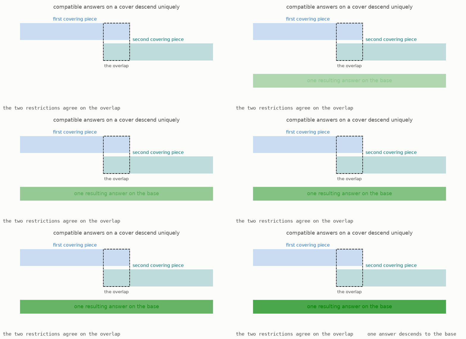
The glue rule requires both existence and uniqueness. Compatible local answers must produce a global answer, and the same local data cannot produce two different global answers. Together with the cut rule, this gives the definition of a condensed set (Definition 1.2, page 6).
The definition also has a size detail (Remark 1.4, page 7). There are too many profinite sets to place all of them inside one ordinary set. The theory first chooses a sufficiently large size limit, works within it, and then proves that using a larger limit does not change the result. We will leave this set-theoretic bookkeeping in the background.
The mathematics
Definition 1.2, page 6 of the lectures writes the cut rule for disjoint probes as
For the glue rule, begin with a surjection $q:S'\twoheadrightarrow S$ and the projections $p_1,p_2:S'\times_S S'\to S'$. Then
Reading the symbols. The letter $T$ names a condensed set, and $T(S)$ is its set of answers on $S$. The symbol $\sqcup$ means disjoint union, and $\times$ means Cartesian product. An arrow marked $\sim$ means a bijection. The double-headed map $q$ is a cover. The fibre product $S'\times_S S'$ contains pairs of points in the cover that represent the same point below. The maps $p_1$ and $p_2$ choose the first and second point in such a pair. A star in $p_i^*$ means pullback. The braces mean “the set of,” $\in$ means “belongs to,” and the vertical bar means “such that.” The equality requires both representatives of each point to receive the same answer.
Why it matters. The first bijection lets us work independently on separate pieces. The second says that compatible data on a cover come from exactly one answer below. Together with $T(\varnothing)=*$, these statements define a condensed set.
In the simulation. In cut mode, two controls choose the independent entries of $T(S_1)\times T(S_2)$. In glue mode, they choose the two pullbacks $p_1^x$ and $p_2^x$. An answer appears below only when the pullbacks agree.
5 · A quotient that points cannot detect
We can now return to the two real lines. Their probe data differ because a probe can vary continuously in the usual real line in ways that are impossible in the discrete line. In condensed abelian groups, we can take a cokernel of the identity map between them. Call this cokernel $Q$.
On the one-point probe, $Q$ is zero. Both real lines have the same individual values, so nothing remains after the pointwise quotient. A larger probe can give a nonzero result. It can map continuously into the usual line without being locally constant, so that map does not come from the discrete line.
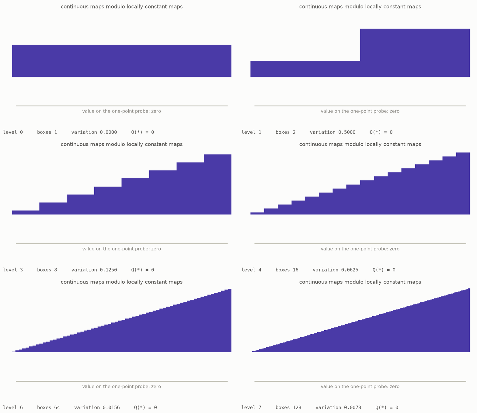
The animation builds a finite approximation to such a map on the halving probe. At each new stage, the values vary on smaller boxes. In the completed probe, a continuous map of this kind never becomes constant on a finite collection of boxes. Every continuous map from a compact probe to a discrete space is locally constant, so this map cannot come from the discrete real line. It represents a nonzero element of $Q$ (Example 1.9, page 9).
This example explains the earlier failure. Individual points could not see the quotient, but a family of nearby points could. Condensed mathematics keeps that missing information as an ordinary algebraic object.
The general theorem says that condensed abelian groups form an abelian category (Theorem 1.10, page 9, with the size limit fixed in Theorem 2.2, page 11). Kernels, cokernels, and exact sequences therefore work together in the expected way.
The mathematics
Example 1.9, page 9 of the lectures identifies the condensed cokernel $Q$ by
The surrounding theorem gives the category in which this cokernel behaves correctly. Theorem 1.10, page 9 states, in particular, that
Reading the symbols. The letter $Q$ names the cokernel, and $Q(S)$ is what the probe $S$ detects. The notation $C(S,\mathbb{R})$ means continuous real-valued maps. The subscript $\mathrm{lc}$ restricts the denominator to locally constant maps. The slash forms the quotient. The star is the one-point probe. Thus $Q(*)=0$ says that one point detects nothing, while $Q\neq0$ says that the condensed group itself is not zero. The notation $\operatorname{Cond}(\mathrm{Ab})$ means condensed abelian groups. An abelian category is a setting in which kernels, cokernels, and exact sequences obey the usual algebraic rules.
Why it matters. A continuous map that is not locally constant gives a nonzero class in $Q(S)$ even though every class vanishes on the one-point probe. The formula shows exactly which information pointwise algebra had discarded.
In the simulation. The variation control changes a map in $C(S,\mathbb{R})$. At zero variation, the map is locally constant and gives the zero class. With nonzero variation, it changes through every visible refinement and represents the kind of class that survives in $Q(S)$. The activity shows finite stages of the construction rather than proving its infinite continuation.
6 · Probes on which every cover splits
Some probes are especially easy to use. Suppose a probe $S'$ covers another probe $S$, meaning that every point of $S$ has at least one point above it in $S'$. A section chooses one point above every point of $S$. It must also make that choice continuously.
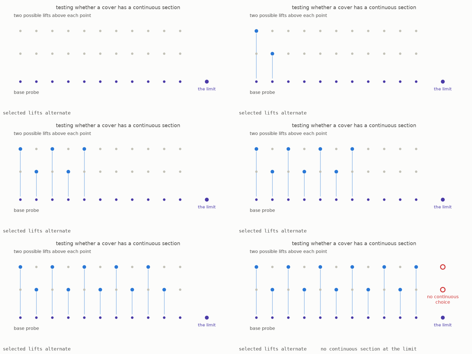
A continuous section does not always exist. In the animation, the choices alternate while the points approach a limit. Choosing either alternating branch forces a jump at the limit. The cover cannot be continuously undone.
A compact Hausdorff probe is extremally disconnected when every cover onto it has a continuous section (Definition 2.4, page 11). One source of these probes is the Stone-Čech compactification of a discrete set. It adds enough limit information so that every map from the original discrete points into a compact space extends continuously. Choosing a lift over each original point and then extending it gives a section (Example 2.5, page 11).
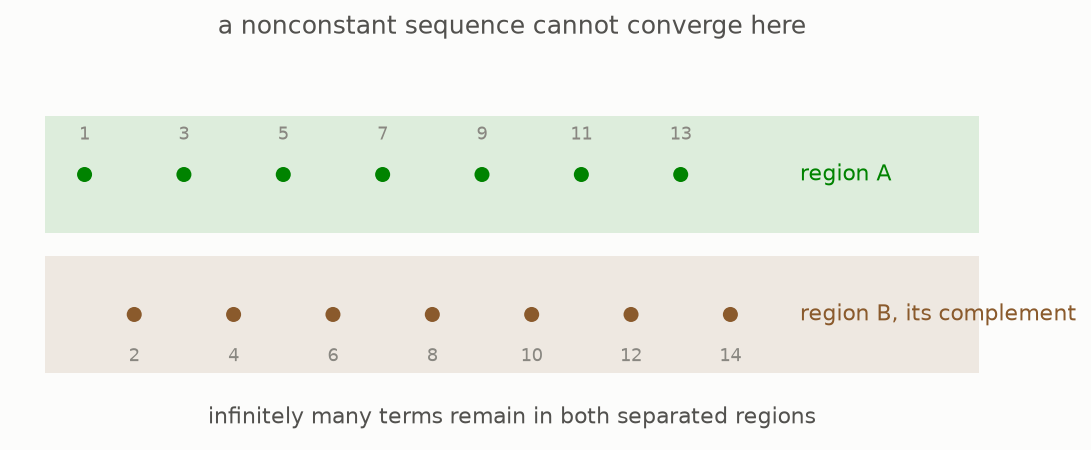
These probes do not behave like familiar geometric spaces. Every convergent sequence in one is eventually constant (Warning 2.6, page 12). If a nonconstant sequence alternated between two groups of terms, the groups could be separated into open-and-closed regions. Infinitely many terms would remain on each side, so the sequence could not converge. The same warning says that a product of two infinite extremally disconnected probes is never extremally disconnected.
Their main advantage comes from the glue rule. Every cover has a section, so compatible data can descend along the section. As a result, a condensed set is determined by its values on these probes, and only the cut rule needs to be checked there (Proposition 2.8, page 12). Parts two and three use these probes as convenient building blocks.
The mathematics
Definition 2.4, page 11 of the lectures says that a compact Hausdorff space $S$ is extremally disconnected when every surjection onto it splits:
Proposition 2.8, page 12 then reduces the conditions for a condensed set on these probes to
The glue condition follows from the fact that every cover splits. A section provides the map needed to bring compatible data back to the original probe.
Reading the symbols. The symbol $\forall$ means “for every,” and $q$ is any surjective map from $S'$ onto $S$. The symbol $\exists$ means “there exists.” The map $s$ is a section, which continuously chooses one point above every point of $S$. The composition $q\circ s$ first goes up by $s$ and then back down by $q$. The expression $\operatorname{id}_S$ is the identity map on $S$, so the equality says that every point returns to itself. The symbol $\varnothing$ is the empty probe, and $*$ is its single possible answer. The symbols $\sqcup$, $\times$, and $\sim$ mean disjoint union, product, and bijection.
Why it matters. A section lets us undo a cover continuously. On extremally disconnected probes, the glue rule follows automatically, so only the rule for finite disjoint unions remains to be checked.
In the simulation. The chosen points define a proposed section $s$. It works only if the choices stay continuous at the limit and satisfy $q\circ s=\operatorname{id}_S$. The extremally disconnected option represents a probe for which some continuous section exists for every cover.
7 · Recovering familiar spaces
Replacing a space by all its probe maps would not help if we could no longer recover ordinary spaces and their continuous maps. A comparison theorem shows that the new description preserves them for a broad and familiar class of spaces.
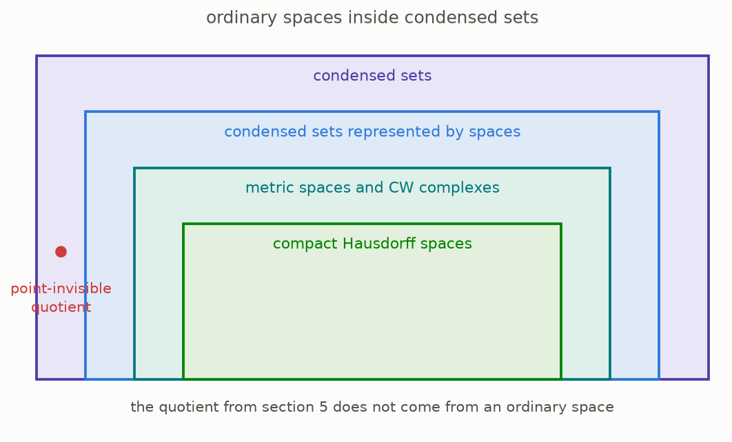
Compact Hausdorff spaces correspond exactly to condensed sets with the matching compactness properties (Theorem 2.16, page 17). Closed and bounded shapes in Euclidean space are standard examples. A larger class, called the compactly generated spaces, includes all metric spaces and spaces built from cells. On this class, the translation is fully faithful: the maps between the condensed descriptions are exactly the original continuous maps (Proposition 1.7, page 9).
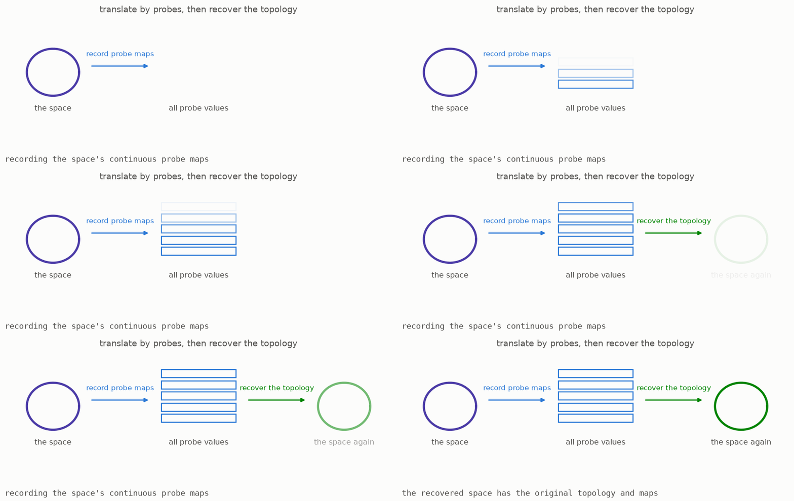
There is also a way back. Start with the point values of a condensed set. Declare a subset closed when every probe detects it as closed. If we begin with a compactly generated space, turn it into probe data, and then apply this rule, we recover the original topology.
The theorem has limits. A topological space with a point that is not closed does not produce a condensed set of the required kind (Warning 2.14, page 16). In the opposite direction, converting a condensed set back into a topological space can lose some information. The lectures give an example involving uncountable increasing unions of compact objects. This does not happen for countable colimits.
The mathematics
Proposition 1.7, page 9 of the lectures says that $X\mapsto\underline X$ is fully faithful on compactly generated spaces:
It also gives the return map. Theorem 2.16, page 17 identifies the compact case:
Reading the symbols. The notation $\operatorname{Hom}$ means the set of maps. The subscript $\mathrm{Top}$ means continuous maps of topological spaces. The expression $\operatorname{Cond}(\mathrm{Set})$ refers to condensed sets. An underline sends a space to its probe data. An arrow marked $\sim$ is a bijection, so each map of condensed sets comes from exactly one continuous map. The expression $\underline X(*)$ reads the value on the one-point probe, and the subscript $\mathrm{top}$ gives it the topology detected by all probes. The symbol $\cong$ means isomorphic. The symbol $\simeq$ means an equivalence of categories. The abbreviation qcqs means quasicompact and quasiseparated.
Why it matters. On the familiar class used here, the translation preserves spaces and all maps between them. Condensed sets enlarge topology instead of replacing it with a description that forgets ordinary spaces.
In the simulation. Choose a circle, interval, or finite set to follow $X\mapsto\underline X\mapsto(\underline X(*))_{\mathrm{top}}$. Each returns with the same topology. The example with a nonclosed point stops at the first step because it does not meet the theorem's assumptions.
8 · Keeping track of holes
We should also check that probe data preserve topological features such as holes. For a circle, draw a closed path and count how many times it travels around the centre. This integer is the winding number. A continuous deformation can change the path's shape, but it cannot change the winding number unless the path breaks.
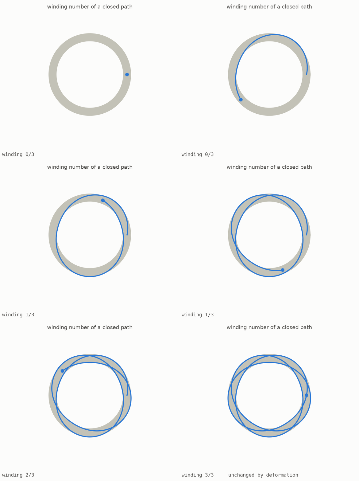
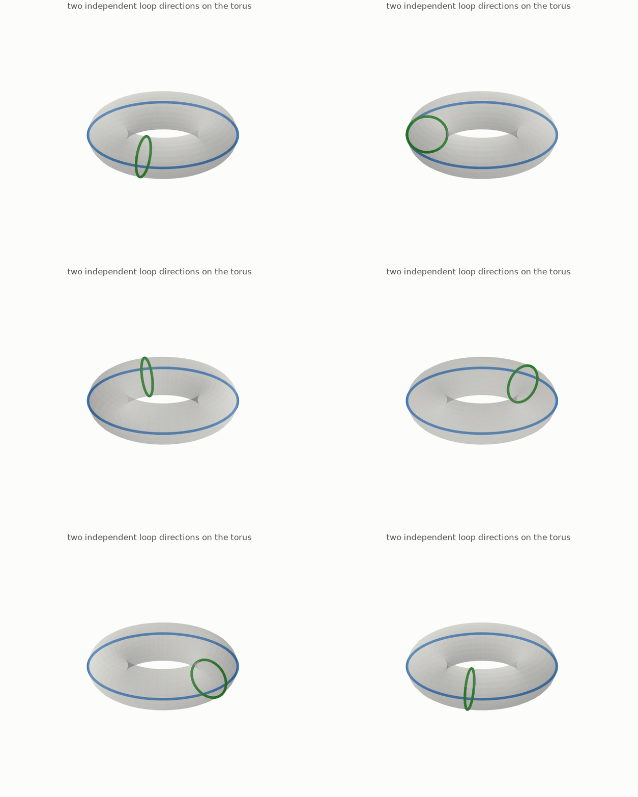
The first cohomology group of a circle is one copy of the integers, and its generator measures this winding number. A product of two circles is a torus. It has two independent loop directions: one passes around the central opening, and one passes around the tube.
Products of more circles have higher-degree holes. We obtain one class by choosing several different circle directions at once. The lectures describe this for any number of circle factors, including infinitely many (Proposition 3.1, page 20).
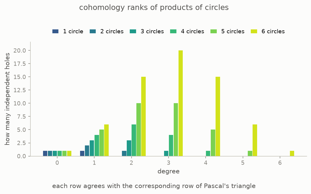
The chart recomputes the finite cases. Each row follows Pascal's triangle because the rank in degree $i$ counts the ways to choose $i$ directions from the available circle directions.
Two results connect this calculation to condensed mathematics. For every compact space, classical sheaf cohomology agrees with cohomology after translation into condensed sets (Theorem 3.2, page 21). With the usual real numbers as coefficients, all positive-degree condensed cohomology vanishes, while degree zero contains the continuous real-valued functions (Theorem 3.3, page 22). This difference between integer and real coefficients will matter in part two.
The mathematics
Let $\mathbb T=\mathbb R/\mathbb Z$ be the circle. Proposition 3.1, page 20 of the lectures computes the cohomology of a product of circles:
Theorems 3.2 and 3.3, pages 21 and 22 compare this with condensed cohomology and describe real coefficients:
Reading the symbols. The circle $\mathbb T$ is the real line $\mathbb R$ with numbers that differ by an integer identified. The product contains one circle for each label $j$ in the index set $I$. The group $H^i$ is cohomology in degree $i$, with integer coefficients $\mathbb Z$. The direct sum $\bigoplus$ contains finite integer combinations of directions. The exterior power $\bigwedge^i$ chooses $i$ distinct directions at a time. The subscripts $\mathrm{sheaf}$ and $\mathrm{cond}$ name classical sheaf cohomology and condensed cohomology. The condition $i>0$ means every positive degree. The notation $C(S,\mathbb R)$ means continuous real-valued functions on $S$.
Why it matters. For $n$ circles, the rank in degree $i$ is $\binom ni$, the number of ways to choose $i$ directions from $n$. The comparison theorem says that the condensed description preserves these hole counts for compact spaces. Real coefficients behave differently because every positive-degree group is zero.
In the simulation. The first control chooses a class in $H^1(\mathbb T,\mathbb Z)$ by setting its winding number. In torus mode, two controls choose the two generators of $H^1(\mathbb T^2,\mathbb Z)$. The displayed ranks $1,2,1$ come from the exterior-power formula.
What part one established
A profinite probe is an inverse system of finite sets. A condensed set records every continuous map from every probe while obeying the cut and glue rules. For familiar spaces, this description preserves the topology, continuous maps, and cohomology. It also detects objects such as $Q$, which are invisible on individual points. This added information makes kernels and cokernels work correctly.
We have not yet defined how to add an infinite family of elements. Such a sum needs a rule for convergence, and different rules can assign different results to the same formal series. Part two builds a summation rule from compatible weights on the finite stages of a probe. The resulting groups are called solid groups.
Part two: Giving Infinite Sums a Meaning
How this part lines up with the lectures
The lectures are stored at docs/condensed-math/paper/lectures-on-condensed-mathematics.pdf and published at arXiv:2605.03658. This table gives the source for each chapter.
| this guide | in the lectures |
|---|---|
| chapter 1, two real lines | Question 1.1 and the problem list, page 6; Example 1.9, page 9 |
| chapter 2, building probes | Definition 1.2, page 6, the profinite sets |
| chapter 3, mapping probes into spaces | Example 1.3, page 7; Remark 1.6, page 9 |
| chapter 4, cut and glue | the two sheaf conditions under Definition 1.2, page 6 |
| chapter 5, the point-invisible quotient | Example 1.9, page 9; Theorem 1.10, page 9; Theorem 2.2, page 11 |
| chapter 6, split covers | Definition 2.4 and Example 2.5, page 11; Warning 2.6 and Proposition 2.8, page 12 |
| chapter 7, recovering spaces | Proposition 1.7, page 9; Warning 2.14, page 16; Theorem 2.16, page 17 |
| chapter 8, cohomology | Proposition 3.1, page 20; Theorem 3.2, page 21; Theorem 3.3, page 22 |
Checking it yourself
You can rebuild the figures and rerun every finite calculation from the repository. You need Python and a command line, but you do not need more mathematical background.
cd condensed-math
make venv        # prepare the software once
make test        # rerun the checked calculations
make figures     # rebuild every picture
For this part, the tests:
- build the three probes as inverse systems and check how their stage sizes grow
- verify that every transition map is surjective and that the maps compose correctly
- check that refining a function does not change its integral against a compatible measure
- run Bergman's finite-stage basis construction and compare the basis size with the number of boxes
- recompute the cohomology ranks of products of circles and confirm the binomial pattern
- calculate winding numbers of sample loops and confirm that deformation does not change them
The program does not prove statements about every object in a category. Results such as the abelian-category theorem and the full-faithfulness theorem are quoted from the lectures. The file notes/research-content.md marks each claim as computed, a finite example of an infinite statement, or quoted.
Glossary
| phrase used in this guide | standard mathematical term |
|---|---|
| a probe | a profinite set |
| a finite stage | one finite set in an inverse system |
| a path through all stages | a point of the inverse limit |
| the halving probe | the Cantor set |
| the approaching-sequence probe | the one-point compactification of the natural numbers |
| the base-$p$ probe | the $p$-adic integers |
| a landing of a probe | a continuous map from the probe to a space |
| the probe data of a space | the condensed set represented by that space |
| a condensed set | a sheaf on the site of profinite sets |
| the discrete real line | the real numbers with the discrete topology |
| the usual real line | the real numbers with their usual topology |
| the point-invisible quotient $Q$ | the cokernel of the discrete reals mapping to the usual reals |
| cut and glue | the sheaf conditions for disjoint unions and surjective covers |
| an extremally disconnected probe | a projective compact Hausdorff space |
| a section | a continuous splitting of a surjection |
| the Stone-Čech completion | the Stone-Čech compactification of a discrete set |
| a hole count | a cohomology group |
| the integer attached to a loop around a circle | the winding number |
Further reading
- Peter Scholze, Lectures on Condensed Mathematics, arXiv:2605.03658, May 2026. The material is joint work with Dustin Clausen. Lectures I to III are the source for this part.
- A. M. Gleason, “Projective topological spaces,” Illinois Journal of Mathematics 2 (1958), for extremally disconnected spaces and their projective property.
notes/research-content.md, for a claim-by-claim record of what is computed and what is quoted.